Cluster Analysis (2)
Classic Clustering Methods
Luc Anselin1
Latest update 11/19/2018
Introduction
In this second of three chapters that deal with multivariate clustering methods, we will cover two classic clustering methods, i.e., k-means, and hierarchical clustering.
The problem addressed by a clustering method is to group the n observations into k clusters such that the intra-cluster similarity is maximized (or, dissimilarity minimized), and the between-cluster similarity minimized (or, dissimilarity maximized). K-means is a so-called partitioning clustering method in which the data are partitioned into k groups, with k determined beforehand. In constrast, hierarchical clustering builds up the clusters from the bottom up (or top down) and can be considered for many values of k.
The clustering methods are standard tools of so-called unsupervised learning and constitute a core element in any machine learning toolbox. An extensive technical discussion is beyond the scope of this document, but a thorough treatment can be found in Hastie, Tibshirani, and Friedman (2009) and James et al. (2013), among others.
GeoDa implements the cluster algorithms by leveraging the C Clustering Library (Hoon, Imoto, and Miyano 2017), augmented by the k-means++ algorithm from Arthur and Vassilvitskii (2007).
To illustrate these techniques, we will continue to use the Guerry data set on moral statistics in 1830 France, which comes pre-installed with GeoDa.
Objectives
-
Carry out k-means clustering
-
Interpret the characteristics of a cluster analysis
-
Carry out a sensitivity analysis to starting options
-
Impose a bound on the clustering solutions
-
Compute aggregate values for the new clusters
-
Carry out hierarchical clustering
GeoDa functions covered
- Clusters > K Means
- select variables
- select k-means starting algorithms
- k-means characteristics
- mapping the clusters
- changing the cluster labels
- saving the cluster classification
- setting a minimum bound
- Clusters > Hierarchical
- select distance criterion
- Table > Aggregate
Getting started
As before, with GeoDa launched and all previous projects closed, we again load the Guerry sample data set from the Connect to Data Source interface. We either load it from the sample data collection and then save the file in a working directory, or we use a previously saved version. The process should yield the familiar themeless base map, showing the 85 French departments, as in Figure 1.
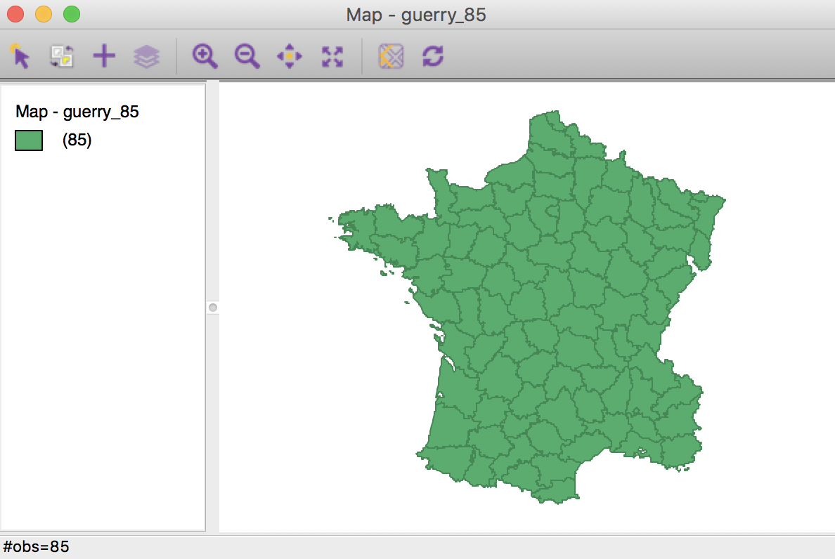
Figure 1: French departments themeless map
K Means
Principle
The k-means algorithm starts with an initial (random) partioning of the n data points into k groups, and then incrementally improves upon this until convergence. In a general sense, observations are assigned to the cluster centroid to which they are closest, using an Euclidean (squared difference) dissimilarity criterion.
A key element in this method is the choice of the number of clusters, k. Typically, several values for k are considered, and the resulting clusters are then compared in terms of the objective function. Since the total variance equals the sum of the within-group variances and the total between-group variance, a common criterion is to assess the ratio of the total between-group variance to the total variance. A higher value for this ratio suggests a better separation of the clusters. However, since this ratio increases with k, the selection of a best k is not straightforward. In practice, one can plot the ratio against values for k and select a point where the additional improvement in the objective is no longer meaningful. Several ad hoc rules have been suggested, but none is totally satisfactory.
The k-means algorithm does not guarantee a global optimum, but only a local one. In addition, it is sensitive to the starting point used to initiate the iterative procedure. In GeoDa, two different approaches are implemented. One uses a series of random initial assignments, creating several initial clusters and starting the iterative process with the best among these solutions. In order to ensure replicability, it is important to set a seed value for the random number generator. Also, to assess the sensitivity of the result to the starting point, different seeds should be tried (as well as a different number of initial solutions).
A second approach uses a careful consideration of initial seeds, following the procedure outlined in Arthur and Vassilvitskii (2007), commonly referred to as k-means++. While generally being faster and resulting in a superior solution in small to medium sized data sets, this method does not scale well (as it requires k passes through the whole data set to find the initial values). Note that a choice of a large number of random initial allocations may yield a better outcome than the application of k-means++, at the expense of a somewhat longer execution time.
Implementation
We invoke the k-means functionality from the Clusters toolbar icon, in Figure 2.
Figure 2: Clusters toolbar icon
We select K Means from the list of options. Alternatively, from the main menu, shown in Figure 3, we can select Clusters > K Means.
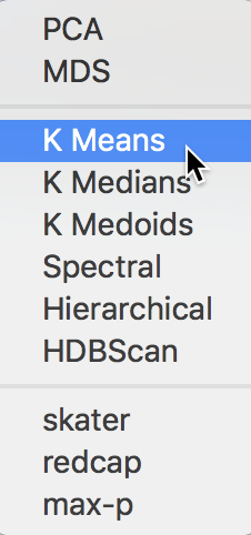
Figure 3: K Means Option
This brings up the K Means Clustering Settings dialog, shown in Figure 4, the main interface through which variables are chosen, options selected, and summary results are provided.
Variable Settings Panel
We select the variables and set the parameters for the K Means cluster analysis through the options in the left hand panel of the interface. We choose the same six variables as in the previous chapter: Crm_prs, Crm_prp, Litercy, Donatns, Infants, and Suicids. These variables appear highlighted in the Select Variables panel.
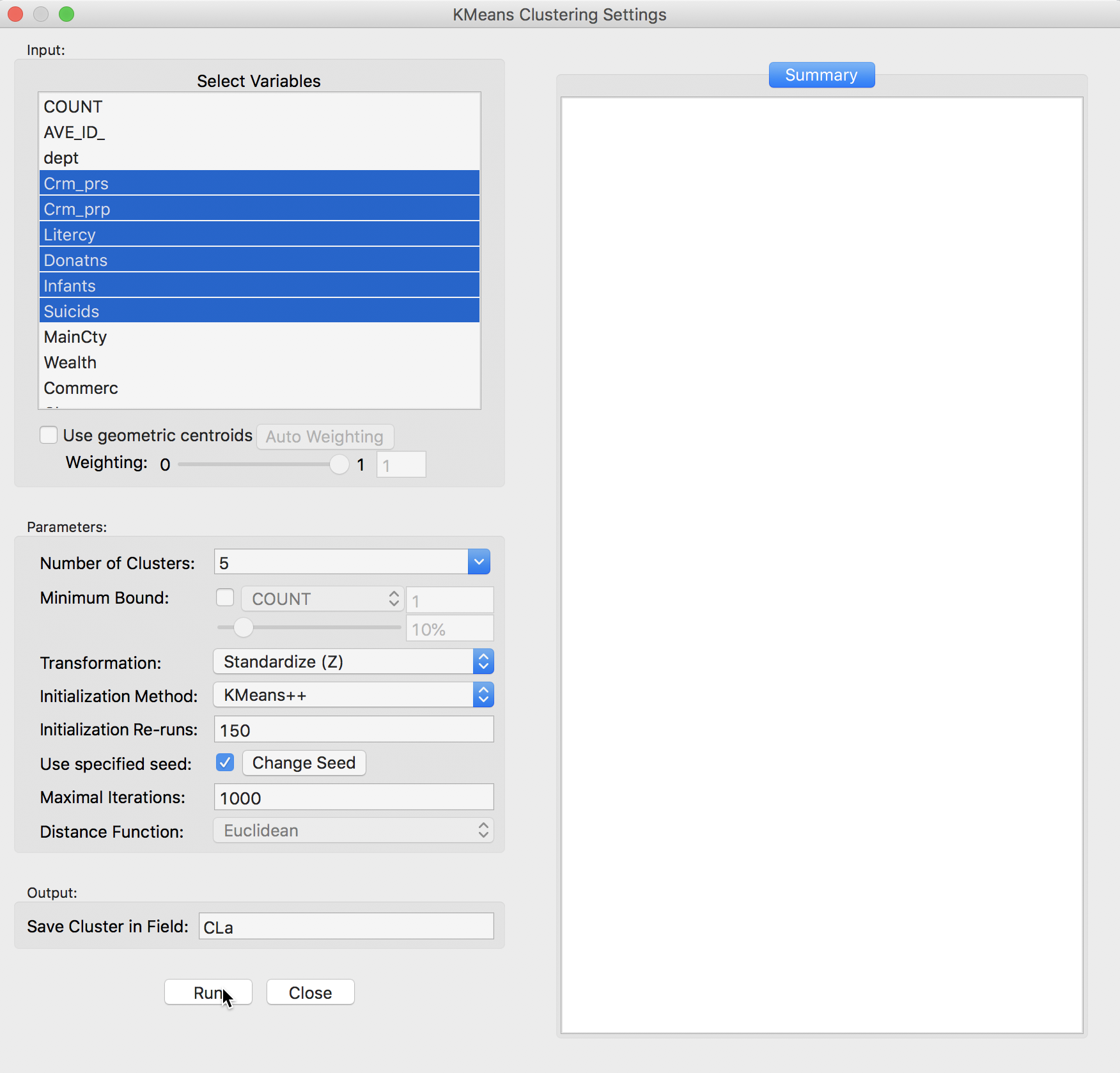
Figure 4: K Means variable selection
The next option is to select the Number of Clusters. The initial setting is blank. One can either choose a value from the drop-down list, or enter an integer value directly.2 In our example, we set the number of clusters to 5.
A default option is to use the variables in standardized form, i.e., in standard deviational units,3 expressed with Transformation set to Standardize (Z).
The default algorithm is KMeans++ with initialization re-runs set to 150 and maximal iterations to 1000. The seed is the global random number seed set for GeoDa, which can be changed by means of the Use specified seed option. Finally, the default Distance Function is Euclidean. For k-means, this option cannot be changed, but for hierarchical clustering, there is also a Manhattan distance metric.
The cluster classification will be saved in the variable specified in the Save Cluster in Field box. The default of CL is likely not very useful if several options will be explored. In our first example, we set the variable name to CLa.
Cluster results
After pressing Run, and keeping all the settings as above, a cluster map is created as a new view and the characteristics of the cluster are listed in the Summary panel.
The cluster map in Figure 5 reveals quite evenly balanced clusters, with 22, 19, 18, 16 and 10 members respectively. Keep in mind that the clusters are based on attribute similarity and they do not respect contiguity or compactness (we will examine this aspect in a later chapter).
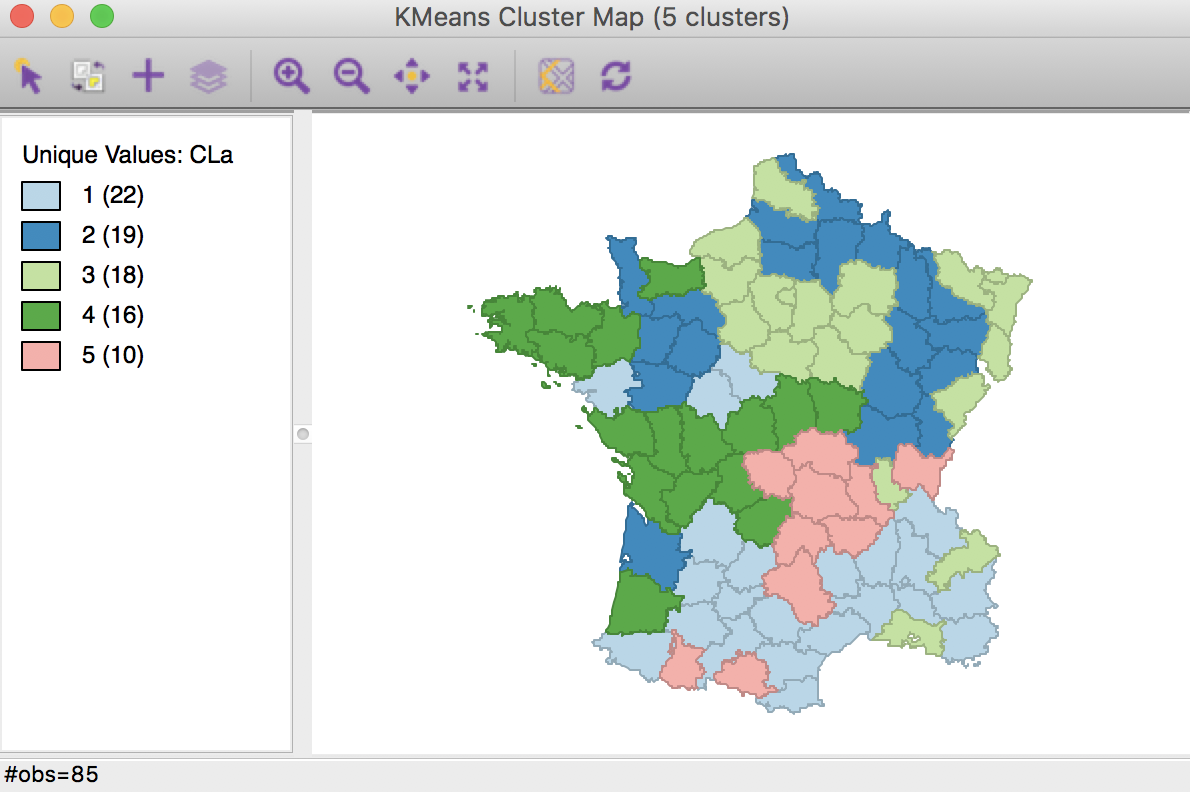
Figure 5: K Means cluster map (k=5)
The cluster characteristics are listed in the Summary panel, shown in Figure 6. This lists, for each cluster, the method (KMeans), the value of k (here, 5), as well as the parameters specified (i.e., the initialization methods, number of initialization re-runs, the maximum iterations, transformation, and distance function). Next follows the values of the cluster centers for each of the variables involved in the clustering algorithm (with the Standardize option on, these variables have been transformed to have zero mean and variance one overall, but not in each of the clusters).
In addition, some summary measures are provided to assess the extent to which the clusters achieve within-cluster similarity and between-cluster dissimilarity. The total sum of squares is listed, as well as the within-cluster sum of squares for each of the clusters. Finally, these statistics are summarized as the total within-cluster sum of squares, the total between-cluster sum of squares, and the ratio of between-cluster to total sum of squares. In our initial example, the latter is 0.497467.
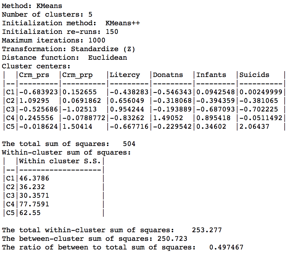
Figure 6: K Means cluster characteristics (k=5)
The cluster labels (and colors in the map) are arbitrary and can be changed in the cluster map, using the same technique we saw earlier for unique value maps (in fact, the cluster maps are a special case of unique value maps). For example, if we wanted to switch category 4 with 3 and the corresponding colors, we would move the light green rectangle in the legend with label 4 up to the third spot in the legend, as shown in Figure 7.
Figure 7: Change cluster labels
Once we release the cursor, an updated cluster map is produced, with the categories (and colors) for 3 and 4 switched, as in Figure 8.
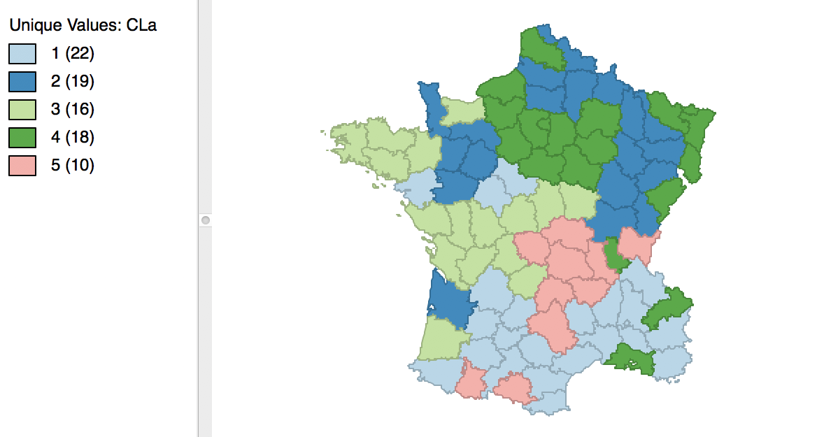
Figure 8: Relabeled cluster map
As the clusters are computed, a new categorical variable is added to the data table (the variable name is specified in the Save Cluster in Field option). It contains the assignment of each observation to one of the clusters as an integer variable. However, this is not automatically updated when we change the labels, as we did in the example above.
In order to save the updated classification, we can still use the generic Save Categories option available in any map view (right click in the map). After specifying a variable name (e.g., cat_a), we can see both the original categorical variable and the new classification in the data table.
In the table, shown in Figure 9, wherever CLa (the original classification) is 3, the new classification (cat_a) is 4. As always, the new variables do not become permanent additions until the table is saved.
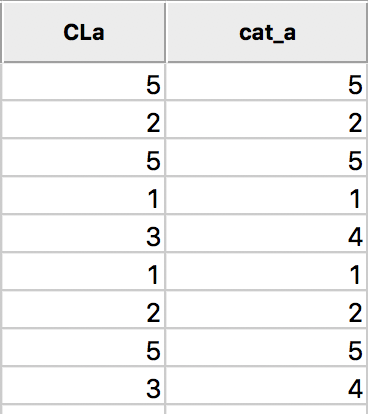
Figure 9: Cluster categories in table
Saving the cluster results
The summary results listed in the Summary panel can be saved to a text file. Right clicking on the panel to brings up a dialog with a Save option, as in Figure 10. Selecting this and specifying a file name for the results will provide a permanent record of the analysis.
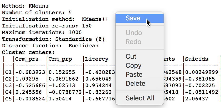
Figure 10: Saving summary results to a text file
Options and sensitivity analysis
The k-means algorithm depends crucially on its initialization. In GeoDa, there are two methods to approach this. The default k-means++ algorithm usually picks a very good starting point. However, the number of initial runs may need to be increased to obtain the best solution.
The second method is so-called random initialization. In this approach, k observations are randomly picked and used as seeds for an initial cluster assignment, for which the summary characteristics are then computed. This is repeated many times and the best solution is used as the starting point for the actual k-means algorithm.
It is important to assess the sensitivity of the results to the starting point, and several combinations of settings should be compared.
In addition to the starting options, it is also possible to constrain the k-means clustering by imposing a minimum value for a spatially extensive variable, such as a total population. This ensures that the clusters meet a minimum size for that variable. For example, we may want to create neighborhood types (clusters) based on a number of census variables, but we also want to make sure that each type has a minimum overall population size, to avoid creating clusters that are too small in terms of population. We will encounter this approach again when we discuss the max-p method for spatially constrained clustering.
Changing the number of initial runs in k-means++
The default number of initial re-runs for the k-means++ algorithm is 150. Sometimes, this is not sufficient to guarantee the best possible result (in terms of the ratio of between to total sum of squares). We can change this value in the Initialization Re-runs dialog, as illustrated in Figure 11 for a value of 1000 iterations.
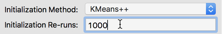
Figure 11: K-means++ initialization re-runs
The result is slightly different from what we obtained for the default setting. As shown in Figure 12, the first category now has 23 elements, and the second 18. The other groupings remain the same.
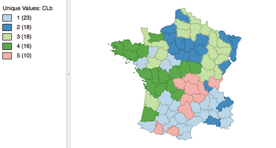
Figure 12: Cluster map for 1000 initial re-runs
The revised initialization results in a slight improvement of the sum of squares ratio, changing from 0.497467 to 0.497772, as shown in Figure 13.
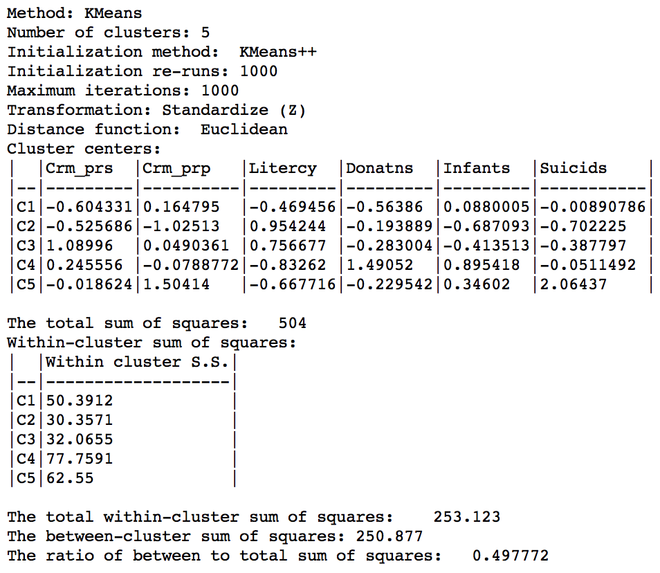
Figure 13: Cluster characteristics for 1000 initial reruns
Random initialization
The alternative to the KMeans++ initialization is to select Random as the Initialization Method, as shown in Figure 14. We keep the number of initialization re-runs to the default value of 150 and save the result in the variable CLr.
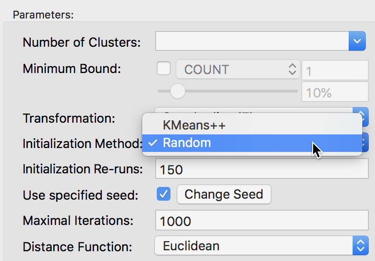
Figure 14: Random initialization
The result is identical to what we obtained for K-means++ with 1000 initialization re-runs, with the cluster map as in Figure 12 and the cluster summary as in Figure 13. However, if we had run the random initialization with much fewer runs (e.g., 10), the results would be inferior to what we obtained before. This highlights the effect of the starting values on the ultimate result.
Setting a minimum bound
The minimum bound is set in the variable settings dialog by checking the box next to Minimum Bound, as in Figure 15. In our example, we select the variable Pop1831 to set the constraint. Note that we specify a bound of 15% (or 4855) rather than the default 10%. This is because the standard k-means solution satisfies the default constraint already, so that no actual bounding is carried out.
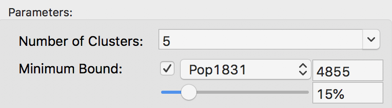
Figure 15: Setting a minimum bound
With the cluster size at 5 and all other options at their default value, we obtain the cluster result shown in the map in Figure 16. These results differ slightly from the unconstrained map in Figure 5.
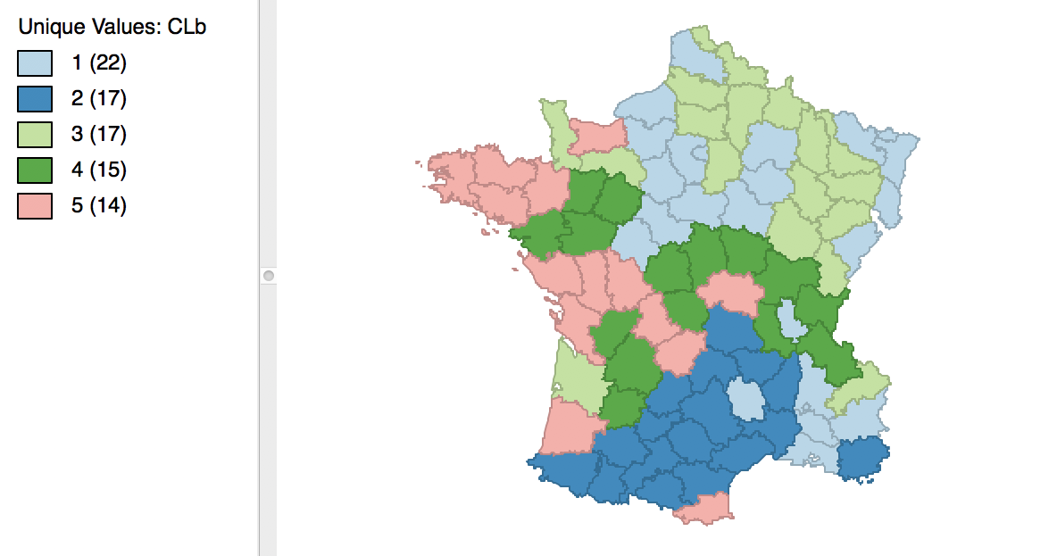
Figure 16: Cluster map with minimum bound constraint
The cluster characteristics show a slight deterioriation of our summary criterion, to a value of 0.484033 (compared to 0.497772), as shown in Figure 17. This is the price to pay to satisfy the minimum population constraint.
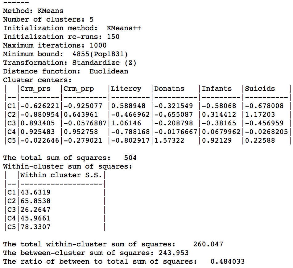
Figure 17: Cluster characteristics with minimum bound
Aggregation by cluster
With the clusters at hand, as defined for each observation by the category in the cluster field, we can now compute aggregate values for the new clusters. We illustrate this as a quick check on the population totals we imposed in the bounded cluster procedure.
The aggregation is invoked from the Table as an option by right-clicking. This brings up the list of options, from which we select Aggregate, as in Figure 18.
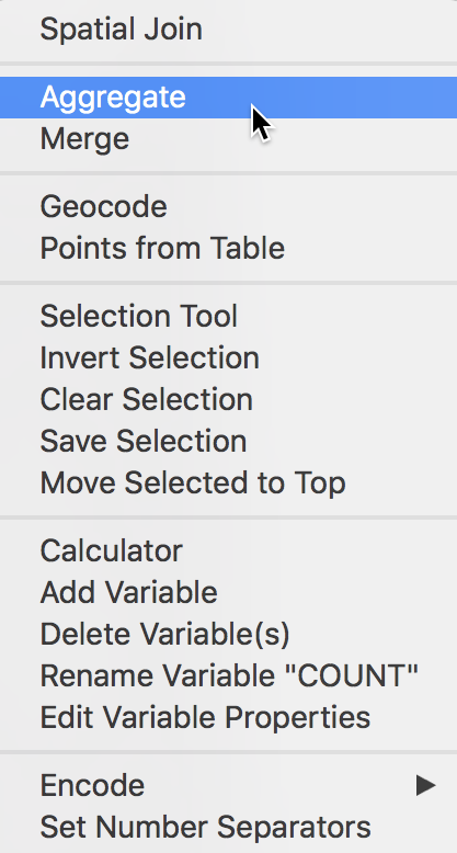
Figure 18: Table Aggregate option
The following dialog, shown in Figure 19, provides the specific aggregation method, i.e., count, average, max, min, or Sum, the key on which to aggregate and a selection of variable to aggregate. In our example, we use the cluster field key, e.g., CLb and select only the population variable Pop1831, which we will sum over the departments that make up each cluster. This can be readily extended to multiple variables, as well as to different summary measures, such as the average.4
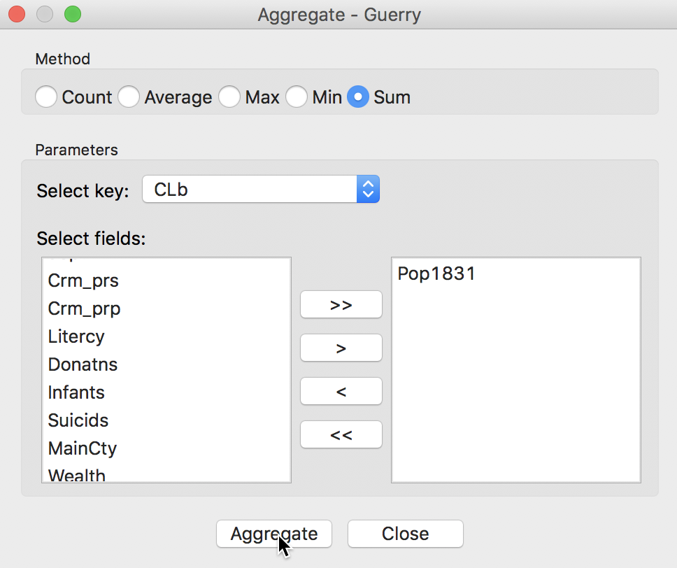
Figure 19: Aggregation of total population by cluster
Pressing the Aggregate key brings up a dialog to select the file in which the new results will be saved. For example, we can select a dbf format and specify the file name. The contents of the new file are given in Figure 20, with the total population for each cluster. Clearly, each cluster meets the minimum requirement of 4855 that was specified.
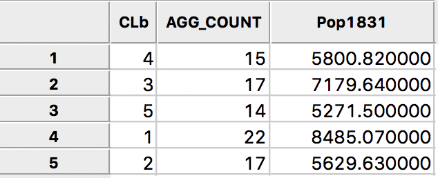
Figure 20: Total population by cluster
The same procedure can be used to create new values for any variable, aggregated to the new cluster scale.
Hierarchical Clustering
Principle
In contrast to a partioning method (like k-means), a hierarchical clustering approach builds the clusters step by step. This can be approached in a top-down fashion or in a bottom-up fashion.
In a top-down approach, we start with the full data set as one cluster, and find the best break point to create two clusters. This process continues until each observation is its own cluster. The result of the successive divisions of the data is visualized in a so-called dendrogram, i.e., a representation as a tree.
The bottom-up approach starts with each observation being assigned to its own cluster. Next, the two observations are found that are closest (using a given distance criterion), and they are combined into a cluster. This process repeats itself, by using a representative point for each grouping once multiple observations are combined. At the end of this process, there is a single cluster, containing all the observations. Again, the results of the sequential grouping of observations (and clusters) are visually represented by a dendrogram.
The dendrogram is used to set a cut level for a specified k. By placing the cut point at different levels in the tree, clusters with varying dimensions are obtained.
A key aspect of the hierarchical clustering process is how to compute the distance between two existing clusters in order to decide how to group the closest two together. There are several criteria in use, such as single linkage, complete linkage, average linkage, and Ward’s method (or centroid linkage).
With single linkage, the distance between two clusters is defined by the distance between the closest (in attribute space) observations from each cluster. In contrast, for complete linkage, the distance is between the observations that are furthest apart. Average linkage uses the average of all the pairwise distances, whereas Ward’s method utilizes the distance between a central point in each cluster.
A common default is to use Ward’s method, which tend to result in nicely balanced clusters. The complete linkage method yields similar clusters. In contrast, single linkage and average linkage tends to result in many singletons and a few very large clusters.
Implementation
Hierarchical clustering is invoked in GeoDa from the same toolbar icon as k-means, shown in Figure 2, by selecting the proper item from the drop down list. The desired clustering functionality can also be selected by using Clusters > Hierarchical from the menu, as shown in Figure 21.
Figure 21: Hierarchical clustering option
Variable Settings Panel
As before, the variables to be clustered are selected in the Variables Settings panel. We continue with the same six variables, shown in Figure 22.
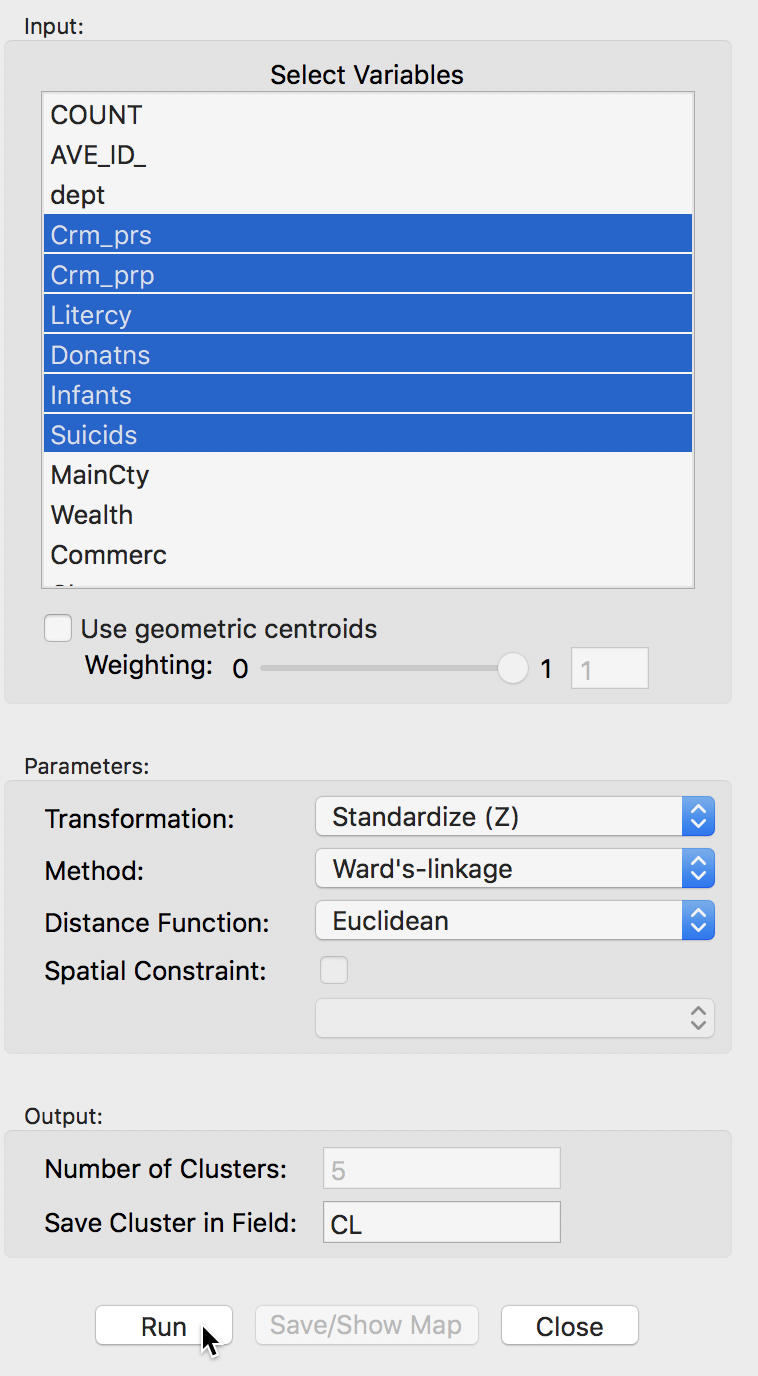
Figure 22: Hierarchical clustering variable selection
The panel also allows one to set several options, such as the Transformation (default value is a standardized z-value), the linkage Method (default is Ward’s method), and the Distance Function (default is Euclidean). In the same way as for k-means, the cluster classification is saved in the data table under the variable name specified in Save Cluster in Field.
Cluster results
The actual computation of the clusters proceeds in two steps. In the first step, after clicking on Run, a dendrogram is presented. The default cut point is set to 5, but this can be changed interactively (see below). Once a cut point is selected, clicking on Save/Show Map creates the cluster map, computes the summary characteristics, and saves the cluster classification in the data table.
Dendrogram
With all options set to the default, the resulting dendrogram is as in Figure 23. The dashed red line corresponds to a cut point that yields five clusters (the default). The dendrogram shows how individual observations are combined into groups of two, and subsequently into larger and larger groups, by combining pairs of clusters. The colors on the right hand side match the colors of the observations in the cluster map (see next).
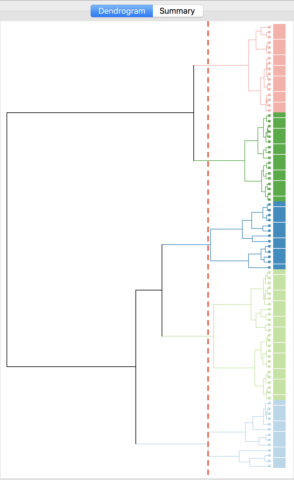
Figure 23: Dendrogram (k=5)
The dashed line (cut point) can be moved interactively. For example, in Figure 24, we grabbed the line at the top (it can equally be grabbed at the bottom), and moved it to the right to yield eight clusters. The corresponding colors are shown on the right hand bar.
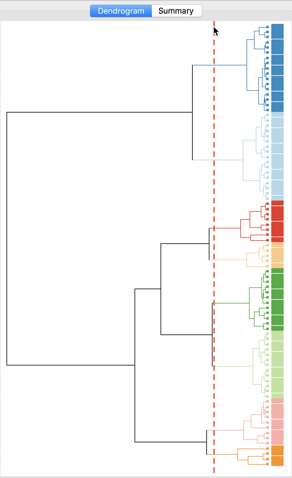
Figure 24: Dendrogram (k=8)
Cluster map
As mentioned before, once the dendrogram cut point is specified, clicking on Save/Show Map will generate the cluster map, shown in Figure 25. Note how the colors for the map categories match the colors in the dendrogram. Also, the number of observations in each class also are the same between the groupings in the dendrogram and the cluster map.
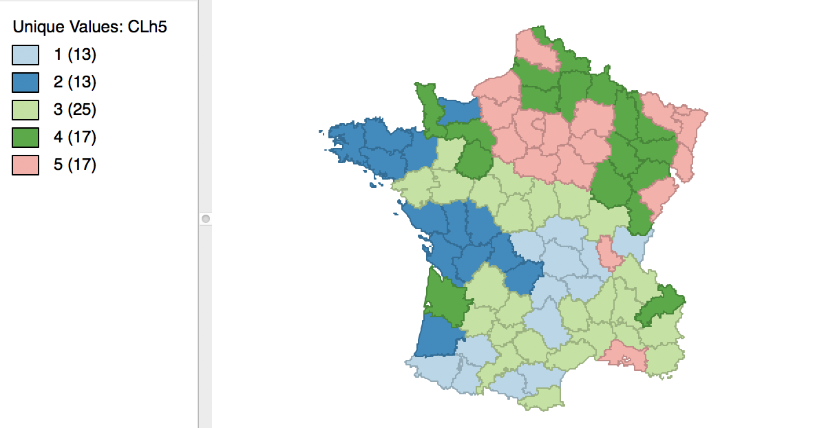
Figure 25: Hierarchical cluster map (Ward, k=5)
Cluster summary
Similarly, once Save/Show Map has been selected, the cluster descriptive statistics become available from the Summary button in the dialog. The same characteristics are reported as for k-means. In comparison to our k-means solution, this set of clusters is slightly inferior in terms of the ratio of between to total sum of squares, achieving 0.482044. However, setting the number of clusters at five is by no means necessarily the best solution. In a real application, one would experiment with different cut points and evaluate the solutions relative to the k-means solution.
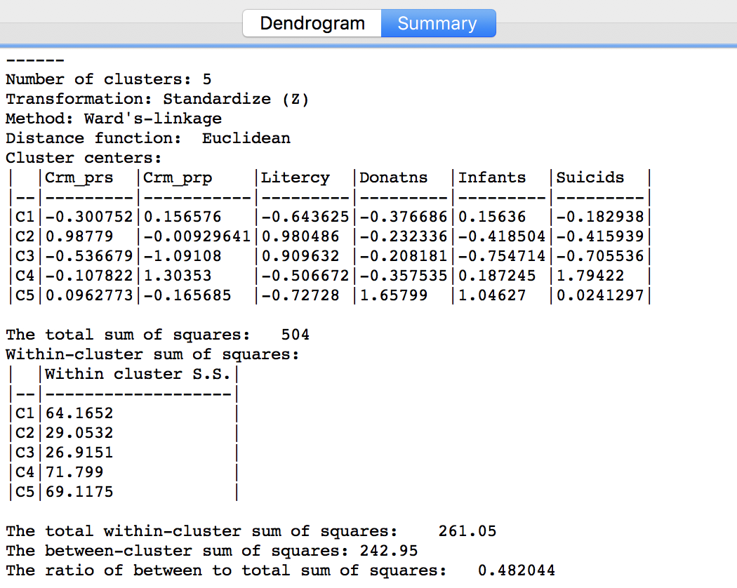
Figure 26: Hierarchical cluster characteristics (Ward, k=5
The two k-means and hierarchical clustering approaches can also be used in conjunction with each other. For example, one could explore the dendrogram to find a good cut-point, and then use this value for k in a k-means or other partitioning method.
Options and sensitivity analysis
The main option of interest in hierarchical clustering is the linkage Method. In addition, we can alter the Distance Function and the Transformation. The latter operates in the same fashion as for k-means.
So far, we have used the default setting for Ward’s-linkage. We now consider each of the other linkage options in turn and illustrate the associated dendrogram, cluster map and cluster characteristics.
Single linkage
The linkage options are chosen from the Method item in the dialog. For example, in Figure 27, we select Single-linkage. The other options are chosen in the same way.
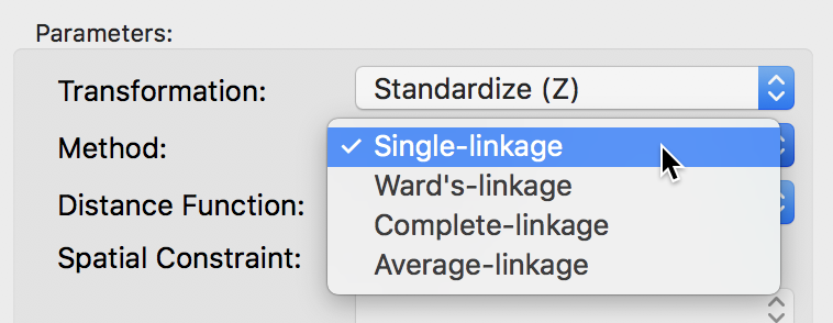
Figure 27: Single linkage
The cluster results for single linkage are typically characterized by one or a few very large clusters and several singletons (one observation per cluster). In our example, this is illustrated by the dendrogram in Figure 28, and the corresponding cluster map in Figure 29. Four clusters consist of a single observation, with the main cluster collecting the 81 other observations. This situation is not remedied by moving the cut point such that more clusters result, since almost all of the additional clusters are singletons as well.
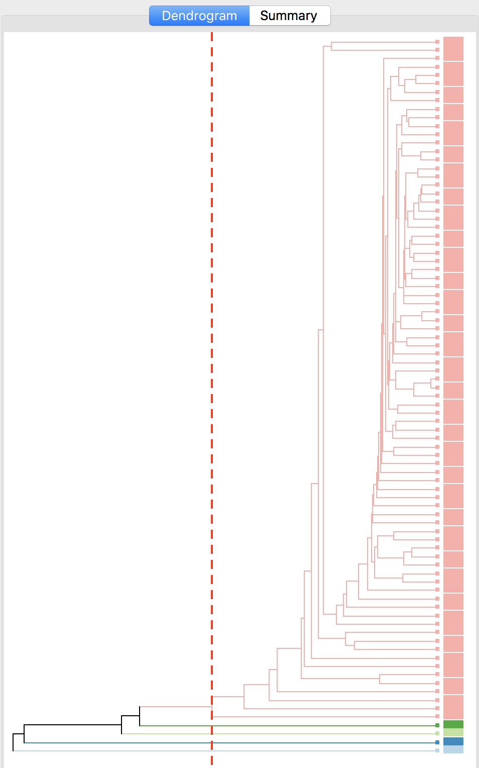
Figure 28: Dendrogram single linkage (k=5)
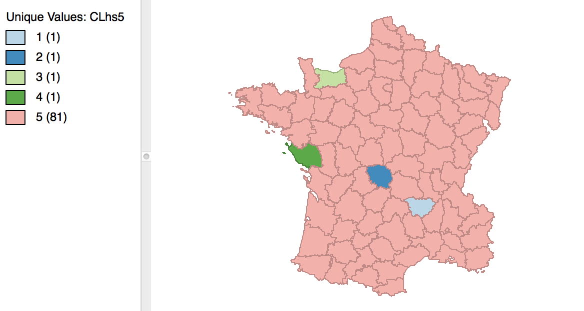
Figure 29: Hierarchical cluster map (single linkage, k=5)
The characteristics of the single linkage hierarchical cluster are similarly dismal. Since four clusters are singeltons, their within cluster sum of squares is 0. Hence, the total within-cluster sum of squares equals the sum of squares for cluster 5. The resulting ratio of between to total sum of squares is only 0.214771.
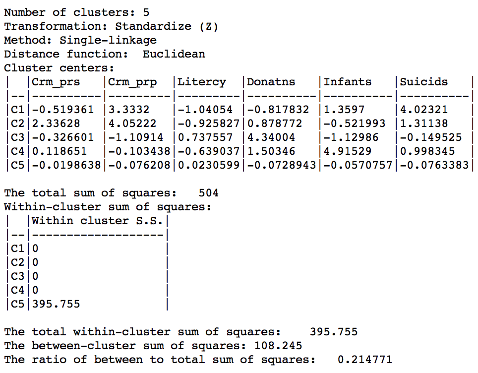
Figure 30: Hierarchical cluster characteristics (single linkage, k=5)
In practice, in most situations, single linkage will not be a good choice, unless the objective is to identify a lot of singletons.
Complete linkage
The complete linkage method yields clusters that are similar in balance to Ward’s method. For example, in Figure 31, the dendrogram is shown for our example, using a cut point with five clusters. The corresponding cluster map is given as Figure 32. The map is similar in structure to that obtained with Ward’s method (Figure 25), but note that the largest category (at 39) is much larger than the largest for Ward (25).
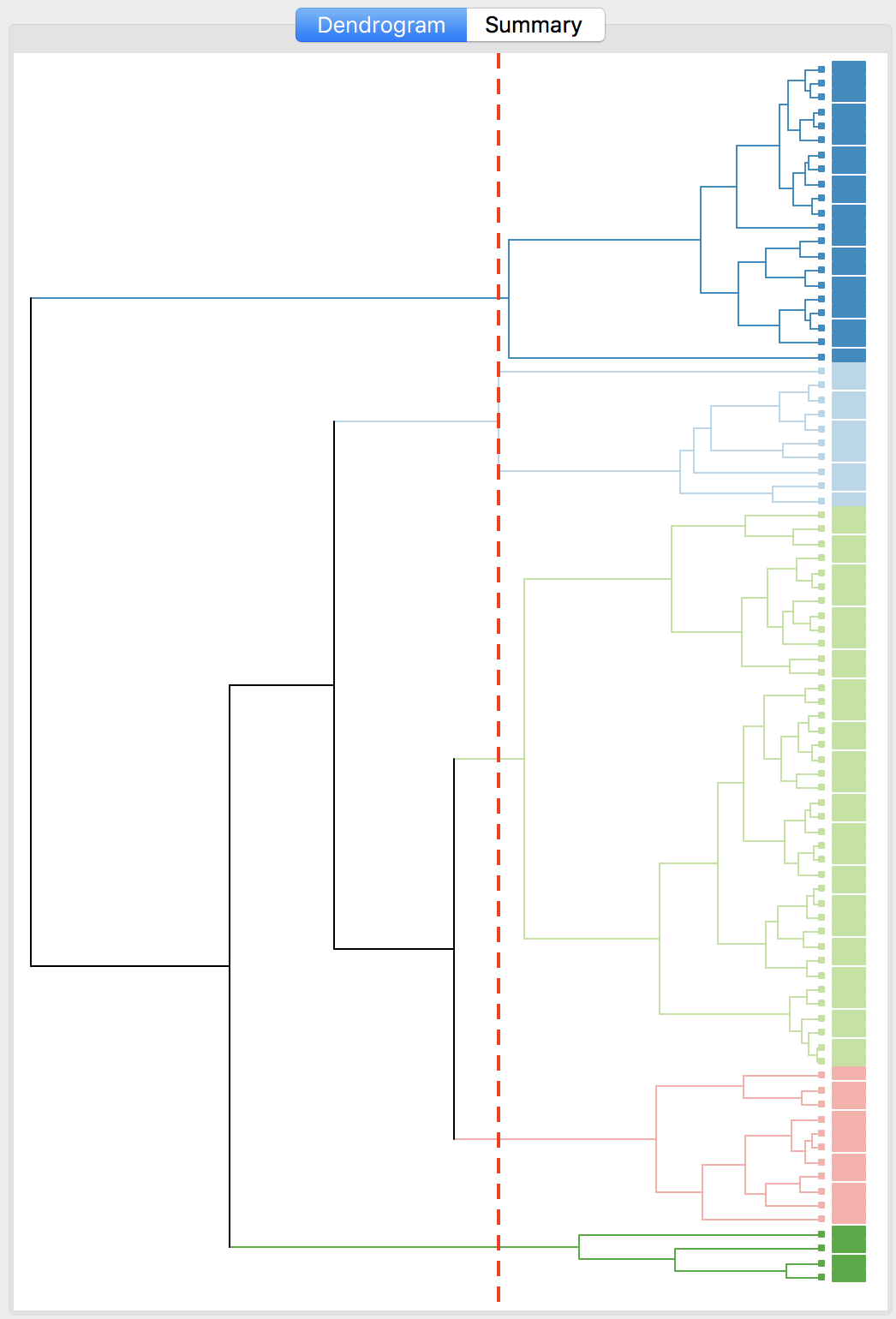
Figure 31: Dendrogram complete linkage (k=5)
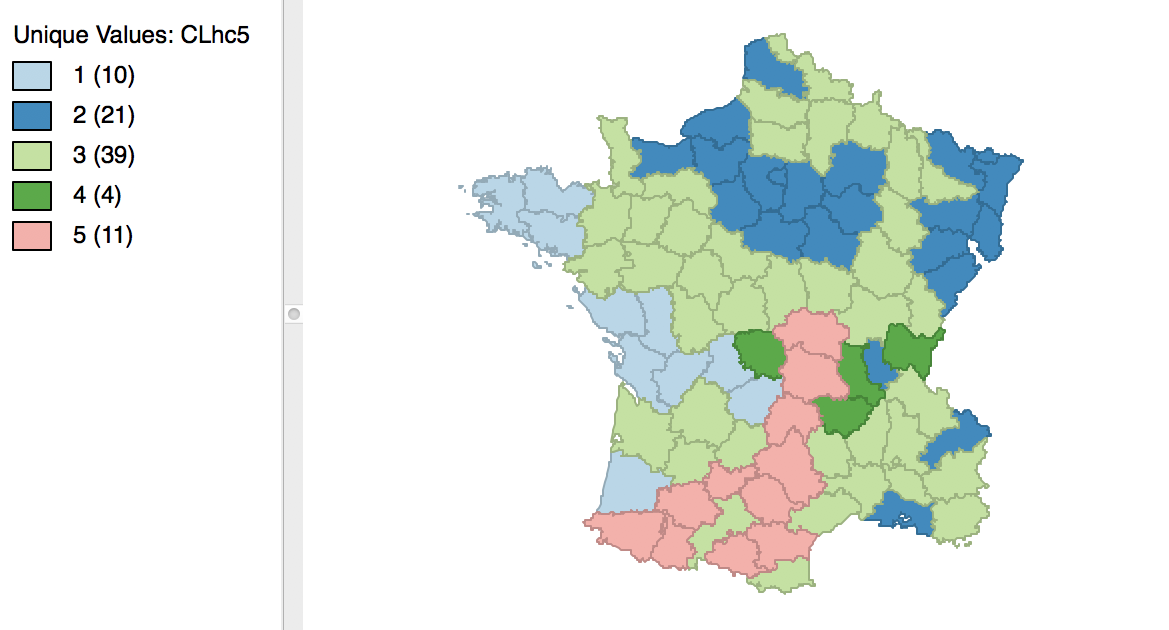
Figure 32: Hierarchical cluster map (complete linkage, k=5)
In terms of the cluster characteristics, shown in Figure 33, we note a slight deterioration relative to Ward’s results, with the ratio of between to total sum of squares at 0.423101 (but much better than single linkage).
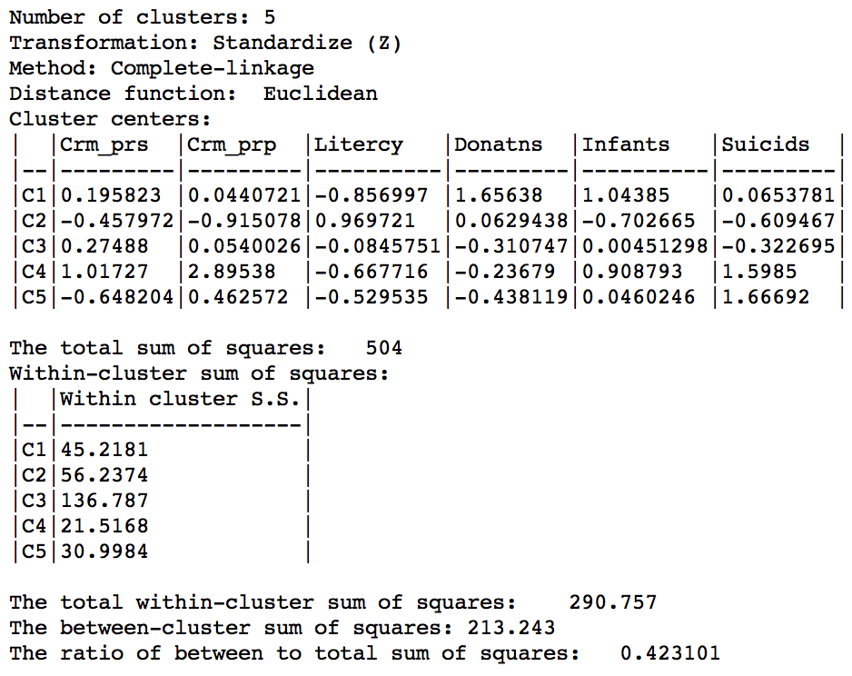
Figure 33: Hierarchical cluster characteristics (complete linkage, k=5)
Average linkage
Finally, the average linkage criterion suffers from some of the same problems as single linkage, although it yields slightly better results. The dendrogram and cluster map are shown in Figures 34 and 35.
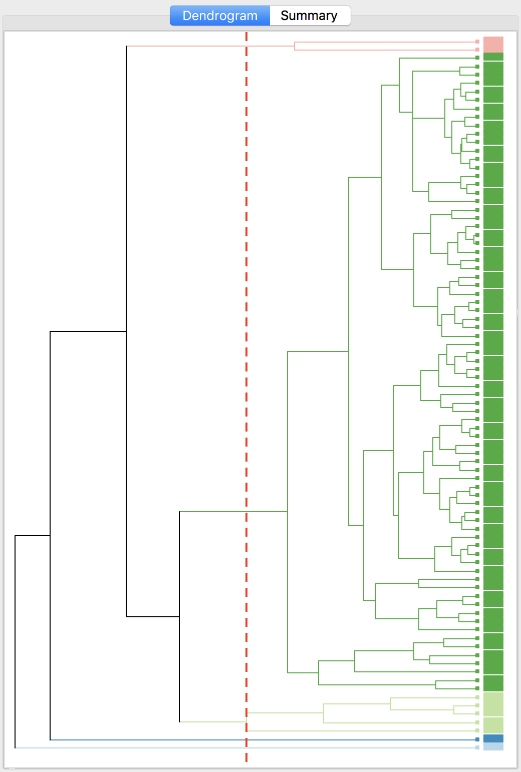
Figure 34: Dendrogram average linkage (k=5)
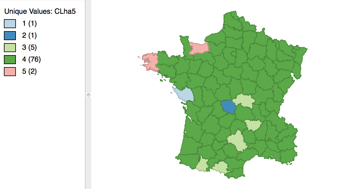
Figure 35: Hierarchical cluster map (average linkage, k=5)
As given in Figure 36, the summary characteristics are slighly better than in the single linkage case, with only two singletons. However, the overall ratio of between to total sum of squares is still much worse than for the other two methods, at 0.296838.
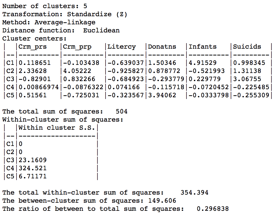
Figure 36: Hierarchical cluster characteristics (average linkage, k=5)
Distance metric
The default metric to gauge the distance between the center of each cluster is the Euclidean distance. In some contexts, it may be preferable to use absolute or Manhattan block distance, which penalizes larger distances less. This option can be selected through the Distance Function item in the dialog, as in Figure 37.
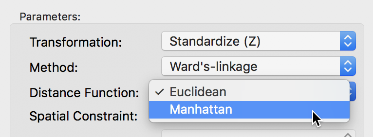
Figure 37: Manhattan distance metric
We run this for the same variables using Ward’s linkage and a cut point yielding 5 clusters. The corresponding cluster map is shown in Figure 38, with the summary characteristics given in Figure 39.
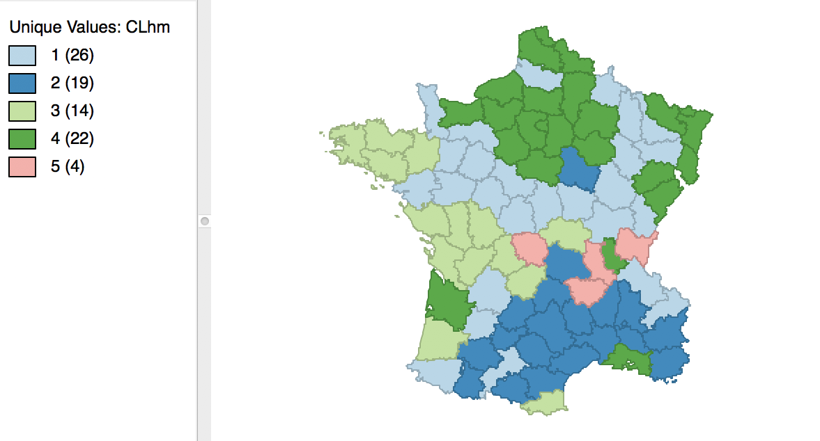
Figure 38: Manhattan distance cluster map
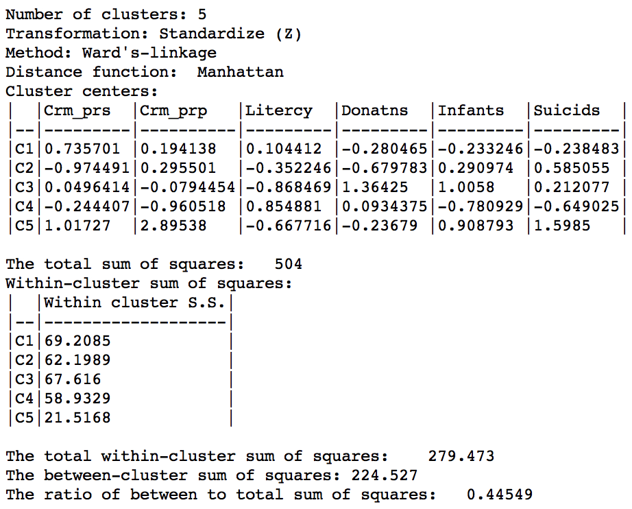
Figure 39: Manhattan distance cluster characteristics
Relative to the Euclidean distance results, the ratio of between to total sum of squares is somewhat worse, at 0.44549 (compared to 0.482044). However, this is not a totally fair comparison, since the criterion for grouping is not based on a variance measure, but on an absolute difference.
References
Arthur, David, and Sergei Vassilvitskii. 2007. “k-means++: The Advantages of Careful Seeding.” In SODA 07, Proceedings of the Eighteenth Annual Acm-Siam Symposium on Discrete Algorithms, edited by Harold Gabow, 1027–35. Philadelphia, PA: Society for Industrial and Applied Mathematics.
Hastie, Trevor, Robert Tibshirani, and Jerome Friedman. 2009. The Elements of Statistical Learning (2nd Edition). New York, NY: Springer.
Hoon, Michiel de, Seiya Imoto, and Satoru Miyano. 2017. “The C Clustering Library.” Tokyo, Japan: The University of Tokyo, Institute of Medical Science, Human Genome Center.
James, Gareth, Daniela Witten, Trevor Hastie, and Robert Tibshirani. 2013. An Introduction to Statistical Learning, with Applications in R. New York, NY: Springer-Verlag.
-
University of Chicago, Center for Spatial Data Science – anselin@uchicago.edu↩
-
The drop-down list goes from 2 to 85, which may be insufficient in big data settings. Hence GeoDa now offers the option to enter a value directly.↩
-
The Z standardization subtracts the mean and divides by the standard deviation. An alternative standardization is to use the mean absolute deviation, MAD.↩
-
In the current implementation, the same summary method needs to be applied to all the variables.↩