Cluster Analysis (3)
Spatially Constrained Clustering Methods
Luc Anselin1
11/28/2017 [in progress, updated]
Introduction
In this lab, we will explore spatially constrained clustering, i.e., when contiguity constraints are imposed on a multivariate clustering method. These methods highlight the tension between the two fundamental criteria behind spatial autocorrelation, i.e., the combination of attribute similarity with locational similarity. To illustrate these techniques, we will continue to use the Guerry data set on moral statistics in 1830 France, which comes pre-installed with GeoDa.
We will consider three methods. One is an extension of k-means clustering that includes the observation centroids (x,y coordinates) as part of the optimization routine, e.g., as suggested in Haining, Wise, and Ma (2000), among others. The other two approaches explicitly incorporate the contiguity constraint in the optimization process. The skater algorithm introduced by Assuncao et al. (2006) is based on the optimal pruning of a minimum spanning tree that reflects the contiguity structure among the observations. The so-called max-p regions model (outlined in Duque, Anselin, and Rey 2012) uses a different approach and considers the regionalization problem as an application of integer programming. In addition, the number of regions is determined endogenously.
Note: the cluster methods in GeoDa are under active development and are not yet production grade. Some of them are quite slow and others do not scale well to data sets with more than 1,000 observations. Also, new methods will be added, so this is a work in progress. Always make sure to have the latest version of the notes.
Objectives
-
Introduce contiguity constraints into k-means clusering
-
Identify contiguous clusters by means of the skater algorithm
-
Identify contiguous clusters with the number of clusters as endogenous with max-p
-
Comparing the characteristics of the clusters
GeoDa functions covered
- Clusters > K Means
- K Means settings
- cluster summary statistics
- cluster map
- introducting geometric centroids
- weighted optimization
- Clusters > Skater
- set minimum bound variable
- set minimum cluster size
- Clusters > Max-p
- set number of iterations
- set initial groups
Getting started
With GeoDa launched and all previous projects closed, we again load the Guerry sample data set from the Connect to Data Source interface. We either load it from the sample data collection and then save the file in a working directory, or we use a previously saved version. The process should yield the familiar themeless base map, showing the 85 French departments.
French departments themeless map
To carry out the spatially constrained cluster analysis, we will need a spatial weights file, either created from scratch, or loaded from a previous analysis (ideally, contained in a project file). The Weights Manager should have at least one spatial weights file included, e.g., Guerry_85_q for first order queen contiguity, as shown here.
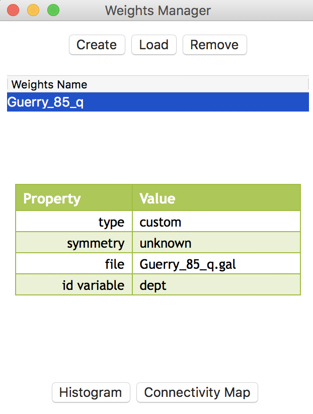
Weights manager contents
K Means with Spatial Constraints
Principle
As we have seen in a previous chapter, the K Means cluster procedure only deals with attribute similarity and does not guarantee that the resulting clusters are spatially contiguous. A number of ad hoc procedures have been suggested to create clusters where all members of the cluster are contiguous, but these are generally unsatisfactory.
An alternative is to include the geometric centroids of the observations as part of the optimization process. There are two general approaches to carry this out. In one, the x and y coordinates are simply added as additional variables in the collection of attributes. While this tends to yield more geographically compact clusters, it does not guarantee contiguity. The second approach consists of a weighted multi-objective optimization, that combines the objective of attribute similarity with that of geometric similarity. This allows for the identification of a cluster with maximal between-cluster dissimilarity that consists of spatially contiguous units.
We consider each approach in turn.
Geometric centroids as attributes
Preliminaries
As we saw in an earier chapter, the K Means procedure is started from the main menu as Clusters > K Means, or from the Clusters toolbar icon.
Before we can proceed, we need to make sure the centroids are part of the data table. Strictly speaking, this is not necessary for the multi-objective optimization (the centroids are computed behind the scenes), but we do need the x, y coordinates in order to include them as part of the attributes to be clustered in the unweighted version.
To this end, we bring up the options menu in the themeless map (or any map), and select Shape Centers > Add Centroids to Table.
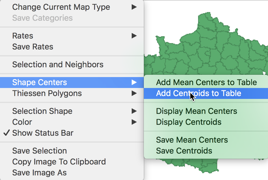
Add centroids to table
We can use the default variable names COORD_X and COORD_Y, or replace them by something more meaningful.
K Means benchmark
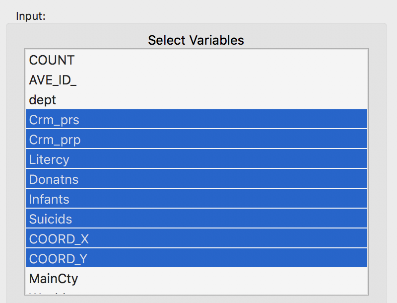
In order to provide a frame of reference, we launch K Means and select the usual six variables (Crm_prs, Crm_prp, Litercy, Donatns, Infants and Suicids) from the Input panel. We leave all other options to the default, except that we set the Number of Clusters to 4. We also set the Field name for the cluster categories to CL_k4, or something similar, so that we can later keep track of all the different cases.
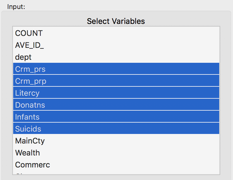
Variables for benchmark case
Clicking on Run generates the cluster map as well as the cluster summary statistics in the Summary panel.2
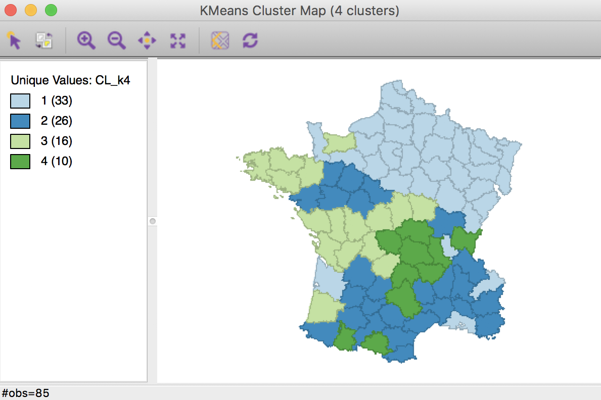
K Means benchmark cluster map (k=4)
The geographic grouping of the observations that are part of each cluster is far from contiguous. The number of disconnected “clusters” ranges from three for group 2 (but note that the labels are arbitrary), to five for group 1.
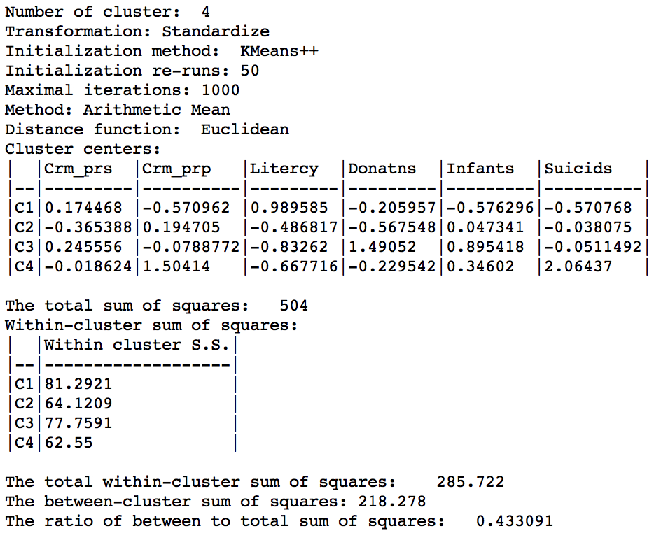
K Means benchmark summary (k=4)
The main descriptive statistic we will use in future comparisons is the ratio of between to total sum of squares, 0.433.
Centroids included as variables
We now repeat the process, but include the two centroids (COORD_X and COORD_Y) among the attributes of the cluster analysis. Again, we set k=4, but keep all other default settings.
Variables for benchmark case
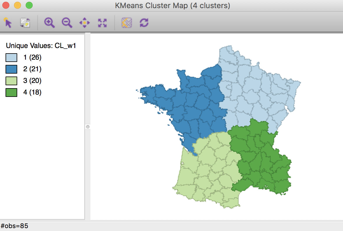
The resulting cluster map is still far from contiguous. Of the four groups, both group 2 and group 3 achieve contiguity among their elements. But group 1 still consists of three parts (including two singletons), and group 4 consists of four parts (including two singletons).
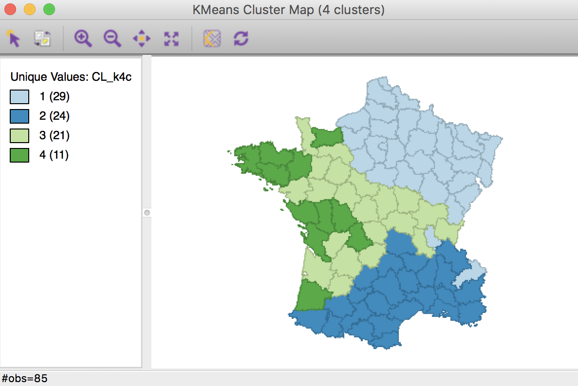
K Means cluster map with centroids (k=4)
The summary now also includes the x, y coordinates of the cluster centers among the descriptive statistics. The overall between cluster dissimilarity increased slightly relative to the base case, to 0.459. Note that this measure now includes the geometric coordinates as part of the dissimilarity measure, so the resulting ratio is not really comparable to the base case.
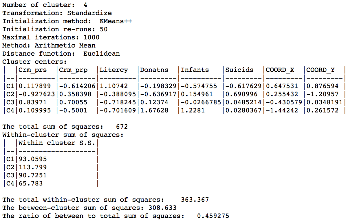
K Means cluster map with centroids summary (k=4)
Weighted optimization
The previous approach included the x and y coordinates as individual variables treated in exactly the same manner as the other attributes (the algorithm does not know that these are coordinates). In contrast, in the weighted optimization, the coordinate variables are treated separately from the regular attributes, in the sense that there are now two objective functions. One is focused on the similarity of the regular attributes (in our example, the six variables), the other on the similarity of the geometric centroids. A weight changes the relative importance of each objective.
To illustrate this, we first consider the case where all the weight is given to the geometric coordinates. We select the same six variables as before, not including the coordinates. In the K-Means Settings dialog, we check the box next to Use geometric centroids. For now, we leave the weight to the value of 1.00. This means that the actual attributes (the six variables) are excluded from the optimization process. The K-Means algorithm is applied to the x, y coordinates only. By setting the weight, the coordinates do not need to be specified explicitly, all the calculations are done in background.

Weighted K Means weights setting
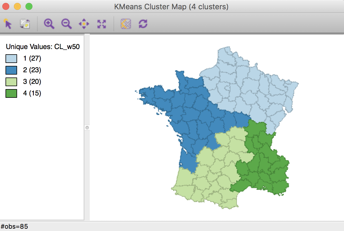
The resulting cluster map shows four compact regions with all members of each cluster contiguous to another member.
Weighted K Means cluster map (w=1,k=4)
Even though the clustering algorithm ignores the actual attributes, the resulting properties can still be calculated. As is to be expected, the results are not that good relative to the pure K-Means. The overall ratio of between to total sum of squares is 0.246, compared to 0.433 in the base case.
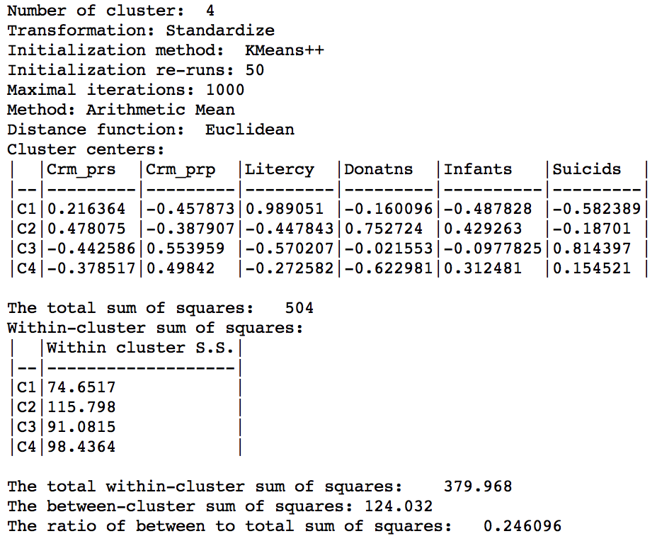
Weighted K Means cluster summary (w=1,k=4)
With the weight set to 0, the same result as in the base case is obtained (not illustrated here). Before moving to an optimization strategy, we check the results with the weight set at 0.5.
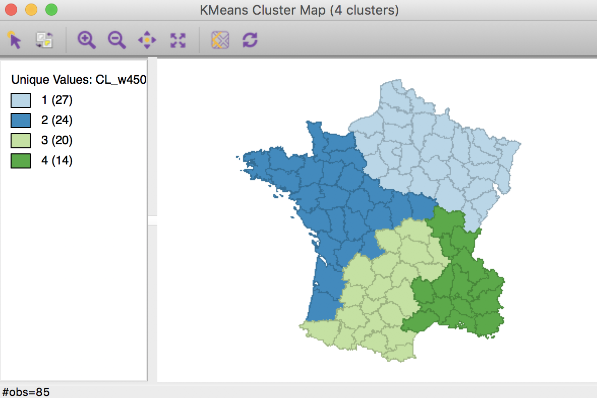
Weighted K Means cluster map (w=0.50,k=4)
The cluster map shows four contiguous subregions, but different from the result obtained in the pure centroid solution.
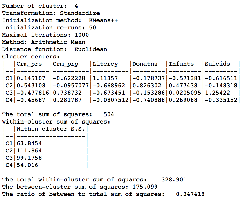
Weighted K Means cluster summary (w=0.50,k=4)
Relative to the pure centroid solution, the overall characteristics have improved substantially, to 0.347 for the between to total sum of squares ratio, but still well below the benchmark a-spatial k-means.
An optimization bisection search
The selection of a value for the weight in the geometric centroids setting constitutes a compromise between attribute similarity (best solution for w=0) and locational similarity (best solution for w=1). We could thus approach the selection of a value for the weight as an optimization problem, where we try to maximize the between to total ratio of the sum of squares, while ensuring contiguity among cluster members.
In a small example like the 85 French departments, we can pursue this manually by means of a bisection search. The logic behind the bisection search is to enclose the optimal solution between an upper and a lower bound for a parameter. At each step, a mid-point is selected that brings us closer to an optimal solution.
In the cluster example, the natural bounds are 0 (pure K-means) and 1 (pure centroids). The midpoint is 0.50. As we just observed, with this value for the weight, the solution is contiguous. This implies that we can do better on the ratio objective by moving closer to the full K-means solution. We thus take as the next value for the weight the midpoint between 0 and 0.50, i.e., 0.25, and check for contiguity.

Weighted K Means cluster map (w=0.25,k=4)
The result has a better ratio of 0.417, but two of the regions no longer have contiguous members, with group 4 consisting of four different sub-regions.
Given that 0.25 does not satisfy the contiguity criterion, we now have to move to the right, to the midpoint between 0.25 and 0.50, or 0.375.
This yields a map that almost meets the contiguity constraint, with a ratio of 0.368. Cluster 1 has one observation that is geographically separated from the rest of the cluster.

Weighted K Means cluster map (w=0.375,k=4)
This means that the next step should be the midpoint between 0.375 and 0.5, or 0.4375. We continue the process until a contiguous solution provides no further meaningful improvement in the sum of squares ratio. In our example, this is for a weight of 0.4500, which yields the following map, with a sum or squares ratio of 0.361.
Weighted K Means cluster map (w=0.4500,k=4)
This is the best we can do in terms of the between to total sum of squares ratio while ensuring contiguity among the members of each cluster. We can now repeat this process for different values of k to assess which combination of number of clusters and centroid weights yields the most satisfactory solution.
Skater
Principle
An approach that explicitly takes into account the contiguity constraints in the clustering process is based on the so-called skater algorithm outlined in Assuncao et al. (2006). The algorithm carries out a pruning of the minimum spanning tree created from the spatial weights matrix for the observations. The weights in the spatial weights matrix correspond to the pair-wise dissimilarity between observations, which become the edges in the graph representation of the weights (the observations are the nodes).
Starting from this weights matrix, a minimum spanning tree is obtained, which is a path that connects all observations (nodes), but each is only visited once. In other words, the n nodes are connected by n-1 edges, such that the between-node dissimilarity is minimized. This tree is then pruned by selecting the edge whose removal increases the objective function (between group dissimilarity) the most. The process continues until convergence. This is a hierarchical process, in that once the tree is cut at one point, all subsequent cuts are limited to the resulting subtrees. In other words, once an observation ends up in a pruned branch of the tree, it cannot switch back to a previous branch. This is sometimes viewed as a limitation of this algorithm.
Implementation
In GeoDa, the skater algorithm is invoked from the Clusters toolbar icon, or from the main menu as Clusters > Skater.
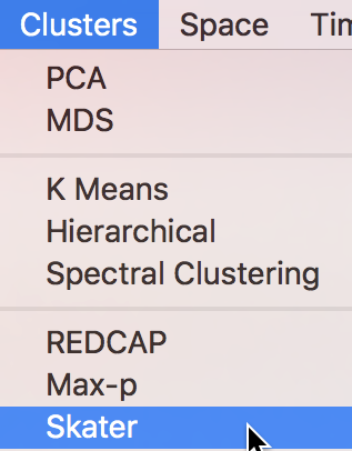
Skater cluster option
Selecting this option brings up the Skater Settings dialog, which has essentially the same structure as the corresponding dialog for K-Means and other classic clustering approaches. The left panel provides a way to select the variables, the number of clusters and different options to determine the clusters. Different from previous approaches is the presence of a Weigths drop down list, where the contiguity weights must be specified. The skater algorithm does not work without a spatial weights file.
The Distance Function, Transformation and seed otpions work in the same manner as for classic clustering. Again, at the bottom of the dialog, we specify the Field or variable name where the classification will be saved.
We consider the Minimum Bound and Min Region Size options below.
We select the same six variables as before: Crm_prs, Crm_prp, Litercy, Donatns, Infants, and Suicids. The spatial weights are based on queen contiguity (Guerry_85_q).
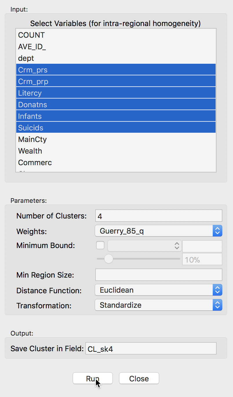
Skater cluster settings
Clicking on Run brings up the skater cluster map as a separate window and lists the cluster characteristics in the Summary panel.
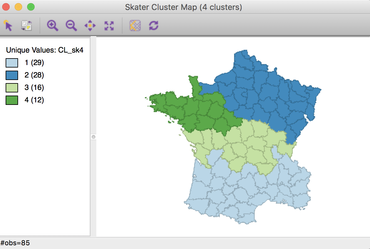
Skater cluster map (k=4)
The spatial clusters generated by skater follow the minimum spanning tree closely and tend to reflect the hierarchical nature of the pruning. In this example, the country initially gets divided into three largely horizontal regions, of which the top one gets split into an eastern and a western part.
The ratio of between sum of squares to total sum of squares is 0.316, somewhat lower than the 0.361 we obtained in the bisection weighted optimization above.
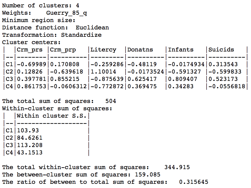
Skater cluster summary (k=4)
The hierarchical nature of the skater algorithm can be further illustrated by increasing the number of clusters to 6 (all other options remain the same). The resulting cluster map shows how the previous regions 2 and 3 each get split into an eastern and a western part.
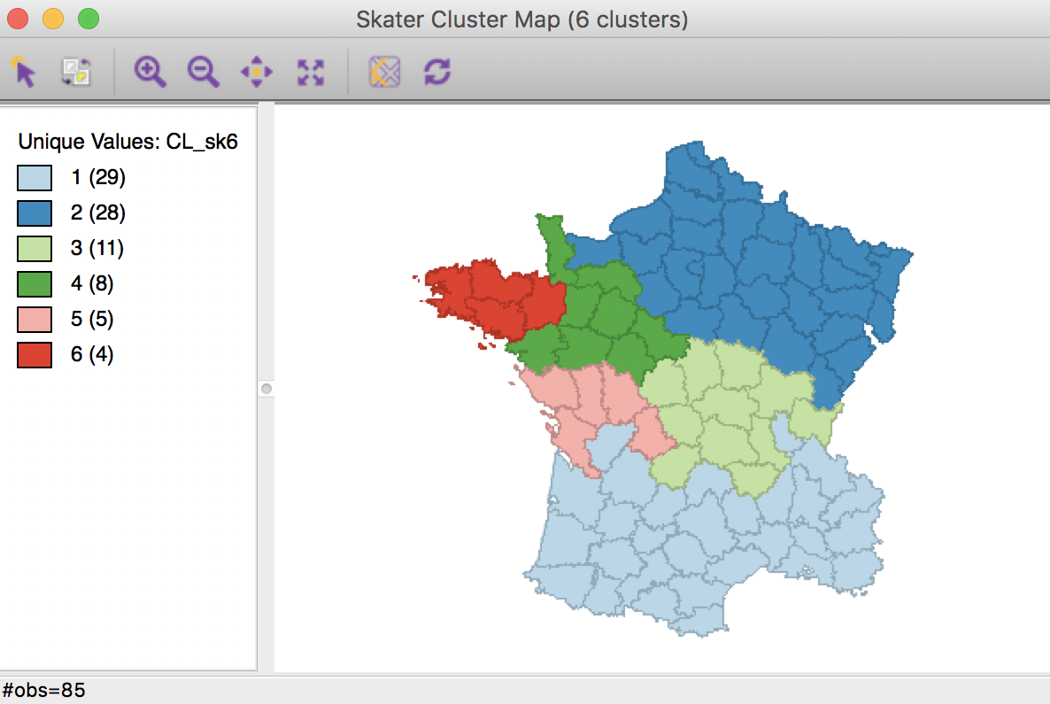
Skater cluster map (k=6)
The ratio of between sum or squares to total sum of squares is now 0.420.
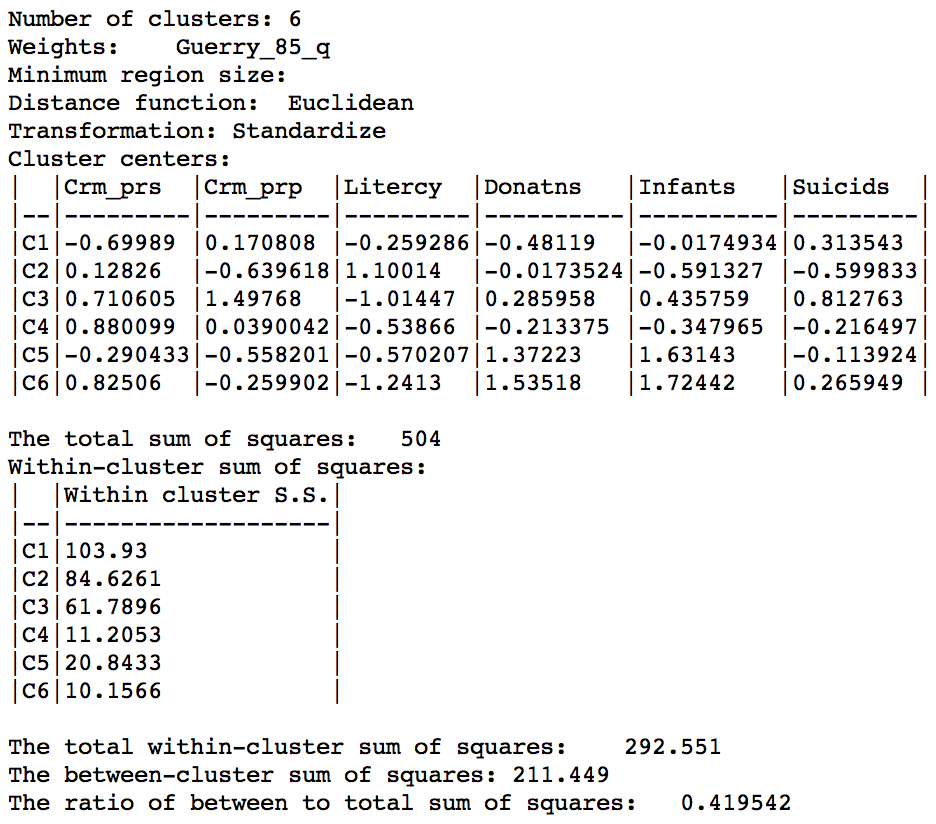
Skater cluster summary (k=6)
Setting a minimum cluster size
In several applications of spatially constrained clustering, a minimum cluster size needs to be taken into account. For example, this is the case when the new regional groupings are intended to be used in a computation of rates. In those instances, the denominator should be sufficiently large to avoid extreme variance instability, which is accomplished by setting a minimum population size.
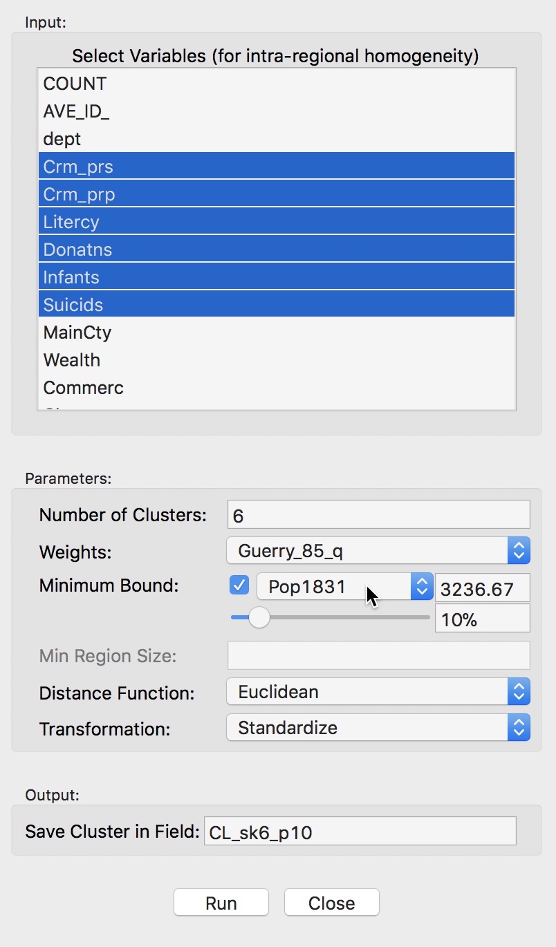
In GeoDa, there are two options to implement this additional constraint. One is through the Minimum Bound settings, as shown below. The check box activates a drop down list of variables where a spatialy extensive variable can be selected for the minimum bound constraint, such as the population (or, in other examples, total number of households, housing units, etc.). In our example, we select the departmental population, Pop1831. The default is to take 10% of the total over all observations as the minimum bound. This can be adjusted by means of a slider bar (to set the percentage), or by typing in a different value in the minimum bound box. Here, we take the default.
Skater minimum bound settings
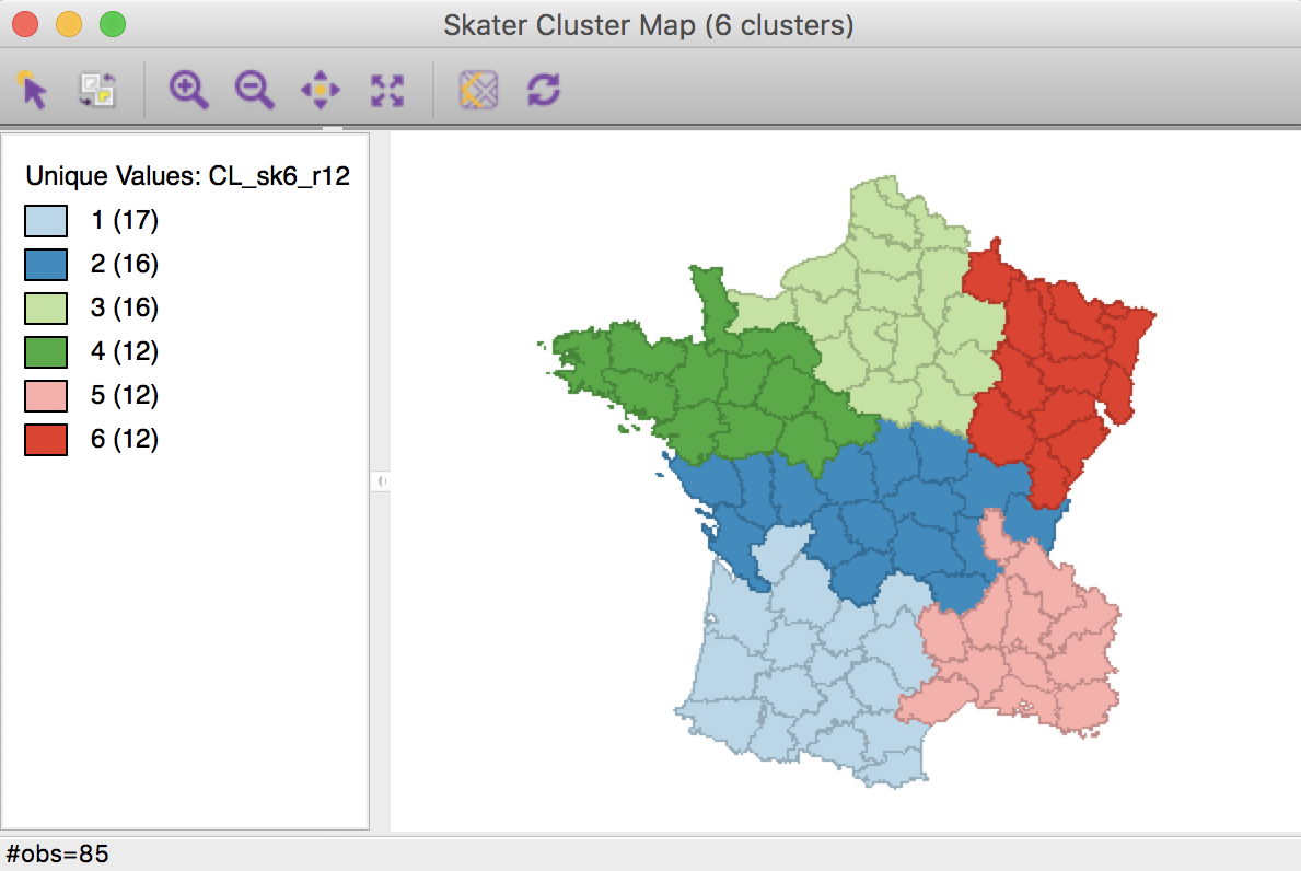
The resulting spatial alignment of clusters is quite different from the unconstrained solution, but again can be seen to be the result of a hierarchical subdivision of the three large horizontal subregions. In this case, the norther most region is divided into three, and the southernmost one into two subregions. Compared to the unconstrained solution, where the clusters consisted of 29, 28, 11, 8, 5, and 4 departments, the constrained regions have a much more even distribution of 17, 16 (twice), and 12 (three times) elements.
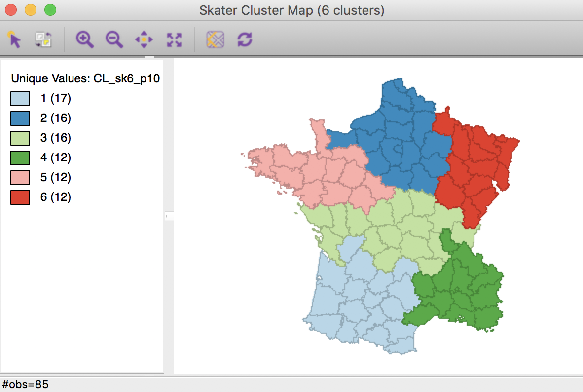
Skater cluster map, min pop 10% (k=6)
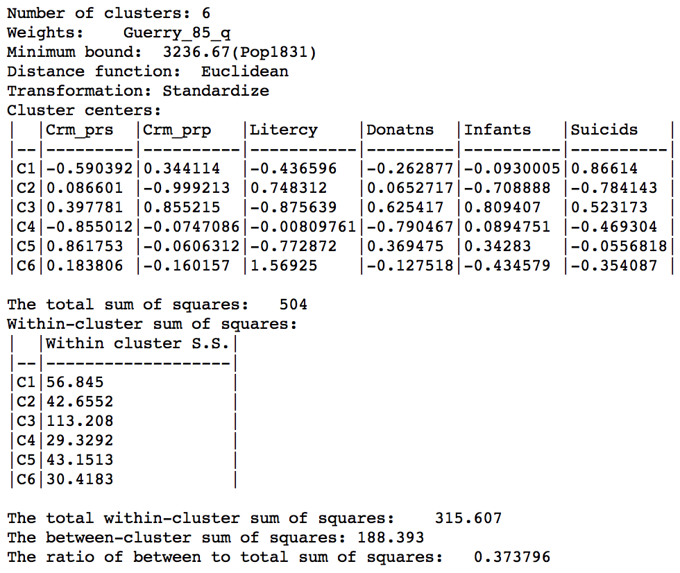
The effect of the constraint is to lower the objective function from 0.420 to 0.374. The within-cluster sum of squares of the six regions is much more evenly distributed than in the unconstrained solution, due to the similar number of elements in each cluster.
Skater cluster summary, min pop 10% (k=6)
The second way to constrain the regionalization process is to specify a minimum number of units that each cluster should contain. Again, this is a way to ensure that all clusters have somewhat similar size, although it is not based on a substantive variable, only on the number of elemental units. The constraint is set in the Min Region Size box of the parameters panel. In our example, we set the value to 12, i.e., the minimum size obtained from the population constraint above.
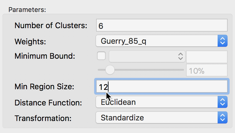
Skater minimum region size settings
The result is identical to that generated by the minimum population constraint, except for the cluster labels (and colors).
Skater cluster map, min size 12 (k=6)
Note that the minimum region size setting will override the number of clusters when it is set too high. For example, setting the minimum cluster size to 14 will only yield clusters with k=5. Again, this is a consequence of the hierarchical nature of the minimum spanning tree pruning used in the skater algorithm. More specifically, a given sub-tree may not have sufficient nodes to allow for further subdivisions that meet the minimum size requirement. A similar problem occurs when the mininum population size is set too high.
Max-p Region Problem
Principle
The max-p region problem, outlined in Duque, Anselin, and Rey (2012), makes the number of regions (k) part of the solution process. This is accomplished by introducing a minimum size constraint for each cluster. In contrast to the skater method, where this was optional, for max-p the constraint is required.
The algorithm itself consists of a search process that starts with an initial feasible solution and iteratively improves upon it while maintaining contiguity among the elements of each cluster. This can take some time, especially for larger data sets. In addition, the iterative process tends to be quite sensitive to the starting point, so an extensive sensitivity analysis is highly recommended.
Implementation
The max-p option is available from the main menu as Clusters > Max-p or as a similarly named option from the Clusters toolbar icon.
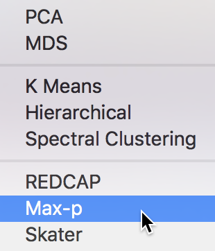
Max-p cluster option
The variable settings dialog is similar to the one for the skater algorithm. We select the same six variables. Also, spatial weights need to be specified in the Weights drop down list (here, we take first order queen contiguity as in Guerry_q_85). In addition, we have to set the MIninum Bound variable and threshold. In our example, we again select Pop1831 and take the 10% default. Finally, we set the number of Iterations to 1000 and leave all other options to their default settings. We specify the Field for the resulting cluster membership as CL_p1k, as shown below.
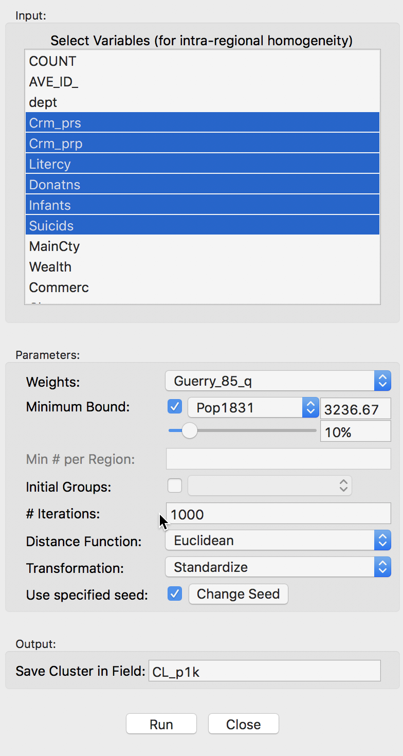
Max-p variables and parameter settings
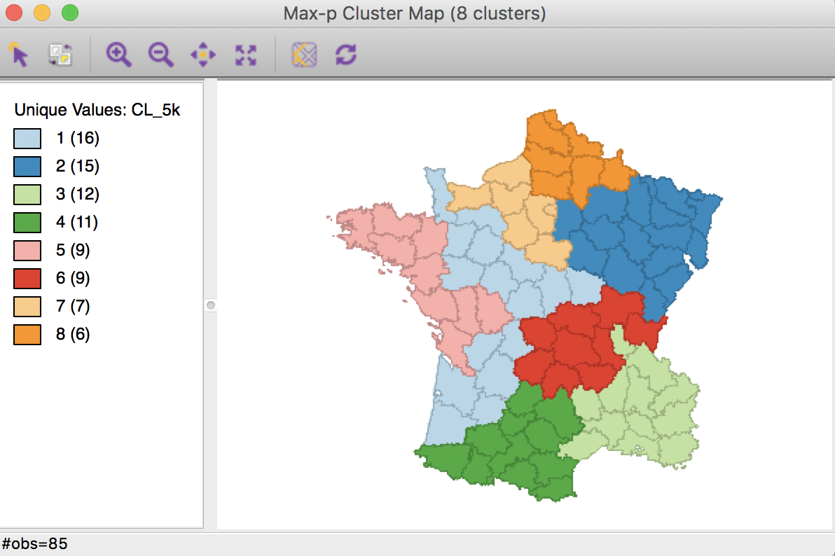
The resulting cluster map yields eight clusters, consisting of 14 to 8 elements.
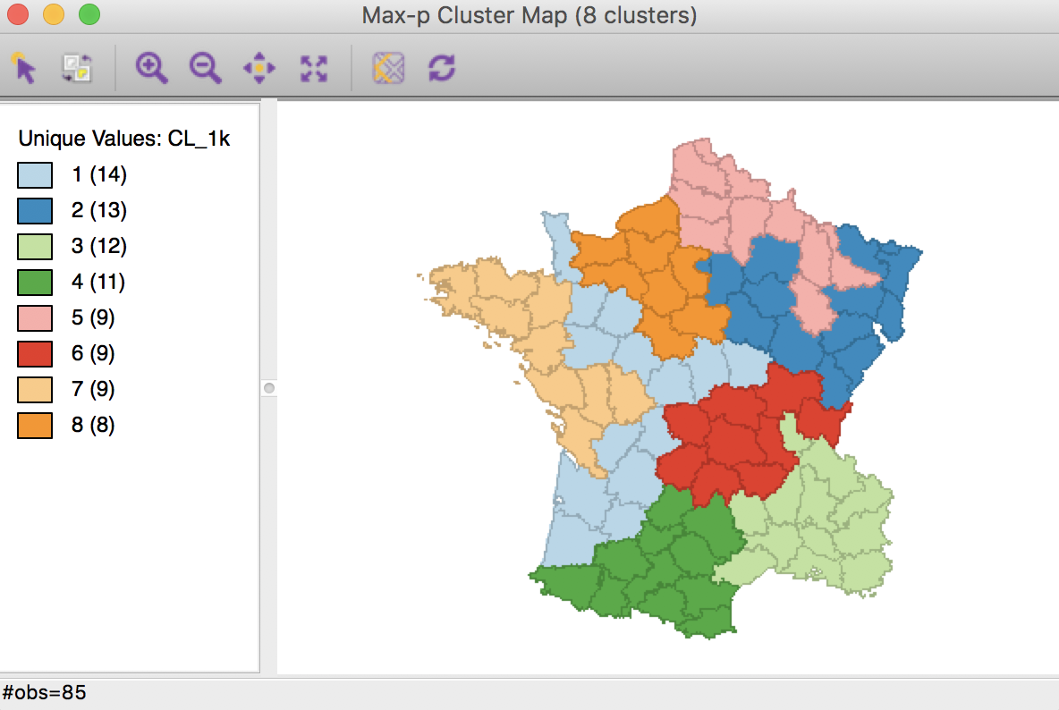
Max-p cluster map, 1000 iterations
The corresponding ratio of between sum of squares to total sum of squares is 0.511. The within sum of squares are fairly evenly distributed, ranging from a low of 11.2 for cluster 5 (9 elements) to a high of 49.2 for cluster 6 (also with 9 elements).
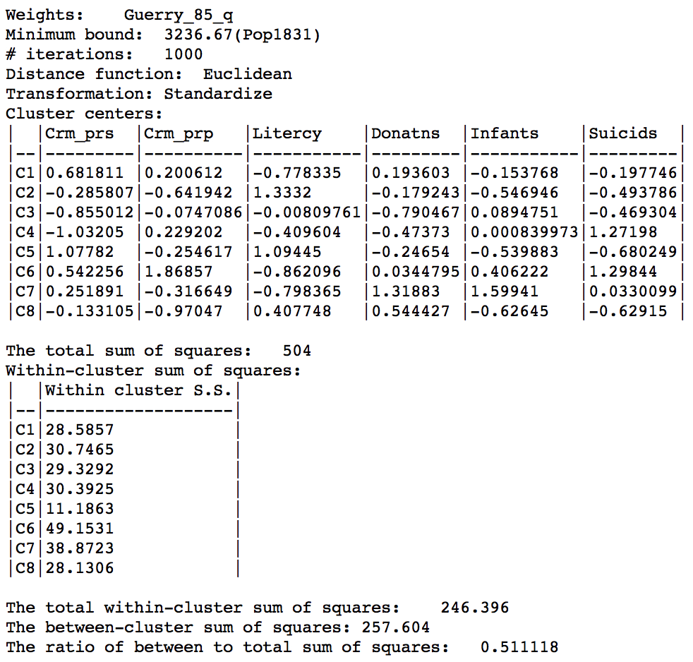
Max-p cluster summary, 1000 iterations
Sensitivity analysis
The max-p optimization algorithm is an iterative process, that moves from an initial feasible solution to a superior solution. However, this process may be slow and can get trapped in local optima. Hence, it behooves us to carry out an extensive sensitivity analysis. There are two main approaches to implement this. One is to increase the number of iterations, starting from the same initial feasible solution. An alternative approach is to adjust the initial feasible solution (the starting point for the search), for example, to start from a solution from an earlier set of iterations. Subsequent iterations may improve on this solution.
The motivation behind the sensitivity analysis is to continue iterating until the resulting solution is stable, i.e., it no longer changes and it reaches a maximum for the objective function.
Changing the number of iterations
The first aspect we consider is to increase the number of iterations. This provides a larger set of alternatives that are considered in the local search process and thereby facilitates moving out of a possible local maximum. For example, we can increase the number of iterations to 5000, which yields the cluster map below. The corresponding ratio of between sum of squares to total sum of squares is 0.519, slightly better than the solution for 1000 iterations (0.511).
Max-p cluster map, 5000 iterations
As it turns out, this solution can be improved upon by increasing the number of iterations to 10000. The associated cluster map is slightly different from the solutions obtained before.
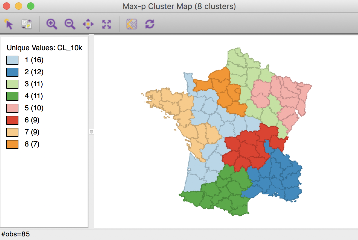
Max-p cluster map, 10000 iterations
The characteristics reveal a very even distribution among clusters, with an overall ratio of between sum of squares to total sum of squares of 0.525, again slightly better.
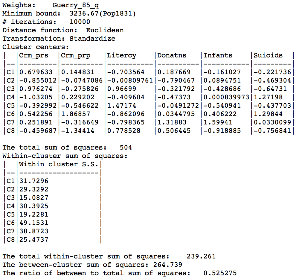
Max-p cluster summary, 10000 iterations
Further increases in the number of iterations do not yield improvements in the objective function. In other words, after 10000 iterations, the same result is obtained, which suggests that the algorithm has yielded a solution that cannot be improved upon with this particular starting point (the default random assignment). However, because of the iterative nature of the algorithm, there is no actual guarantee that a global optimum was obtained.
Setting initial groups
An alternative or complement to increasing the number of iterations is to adjust the starting point for the search. We can specify a feasible initial solution by means of the Initial Groups option in the panel. This refers to a categorical variable that assigns each observation to a cluster. Note this solution has to be feasible, i.e., it must conform to the contiguity constraint. Good candidates for the initial groups are the solutions obtained in an earlier iteration, since these are guaranteed to be feasible. Here, we use the outcome of the 1000 initial iterations, stored in the variable CL_mp1. We set the number of iterations to 10000.
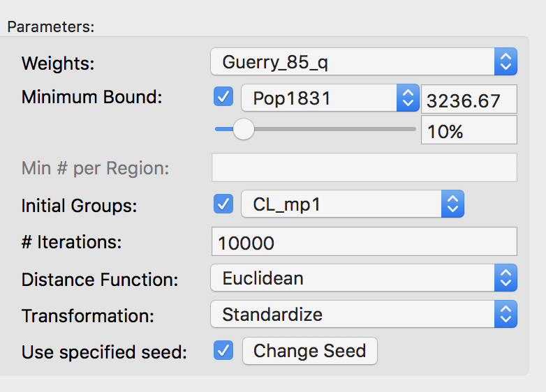
Initial group setting
The result is again slightly different from the previous solution.
In order to make the two maps more comparable, we use the category label switching feature of the unique maps in GeoDa (see the geovisualization chapter) to match the colors and labels of clusters 2, 3 and 4. The resulting cluster map is shown below.
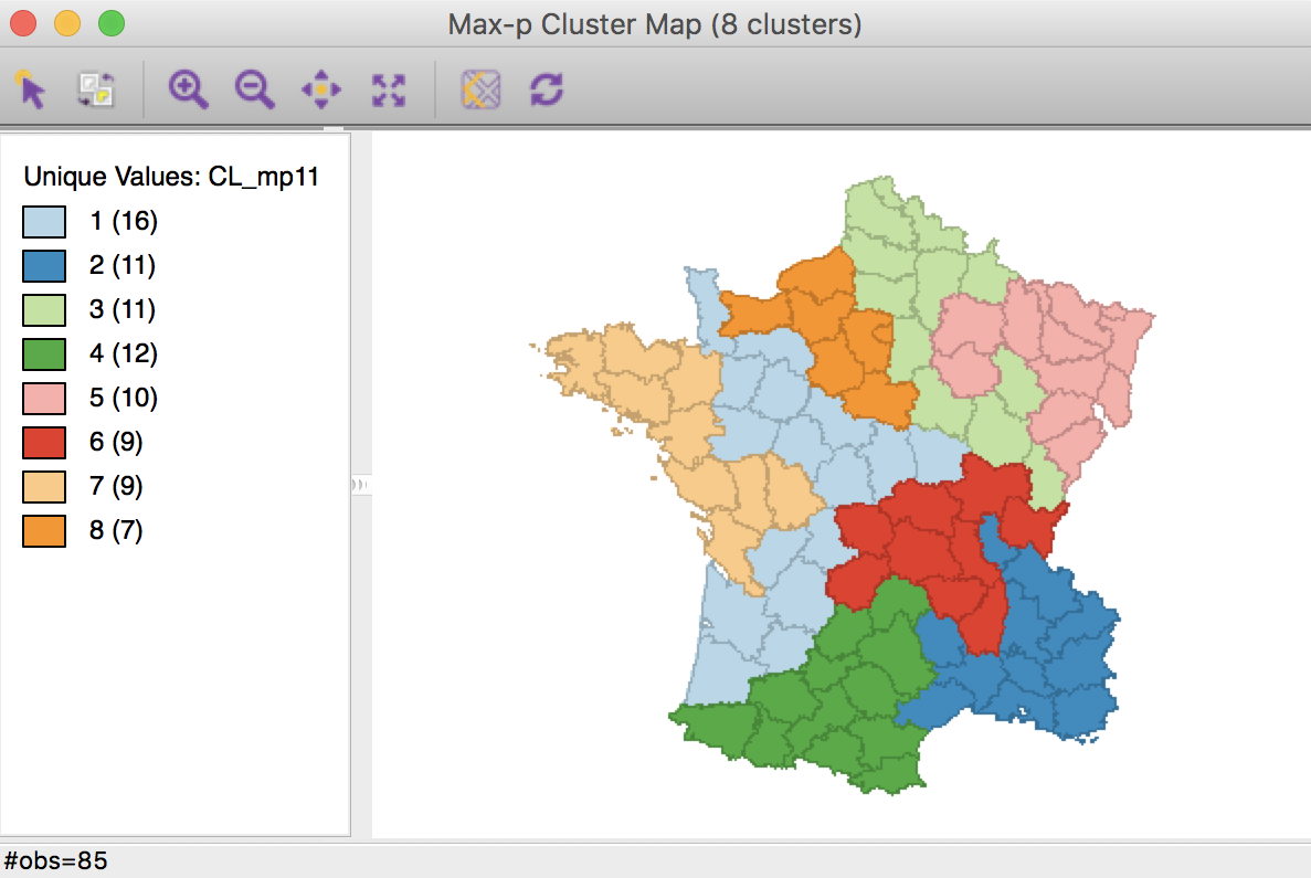
Max-p cluster map, 10000 iterations after CL1k
At first sight, the maps seem the same, with an identical distribution of departments by cluster, except for Cluster 2 (from 12 to 11), as shown in the map legend. Careful examination of the two maps reveals a difference in the allocation of two departments, one moving from Cluster 6 to Cluster 4 (using the new consistent labeling between the two maps), the other moving from Cluster 2 to Cluster 6. This only affects the total in Cluster 2.
We can illustrate this by means of GeoDa’s co-location map. First, we save the categories from the adjusted cluster map (the new categories no longer match the original categorical variable). Then, we create a co-location map for the first cluster map, CL_mp10, and the saved categories, say new_mp11. The resulting unique values map (ignore the color scheme, but the category labels match) clearly shows the two locations that do not match between the two cluster maps.
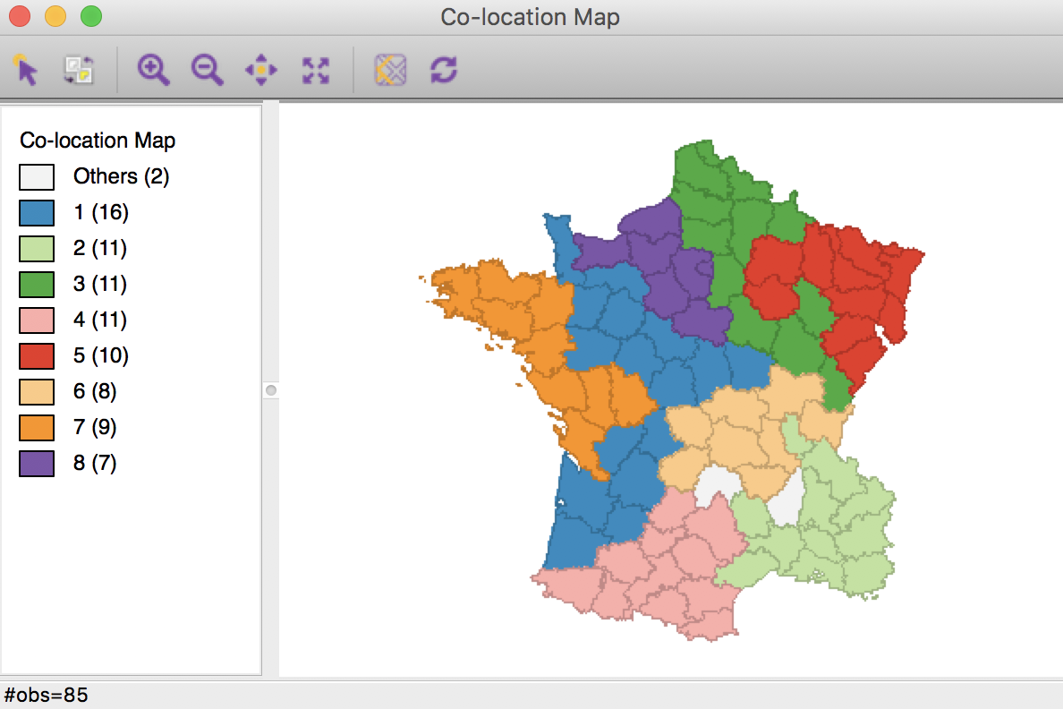
Max-p cluster co-location map
Selecting these locations in the co-location map will also highlight them in the two cluster maps (through the process of linking), which clearly illustrates the two swaps.
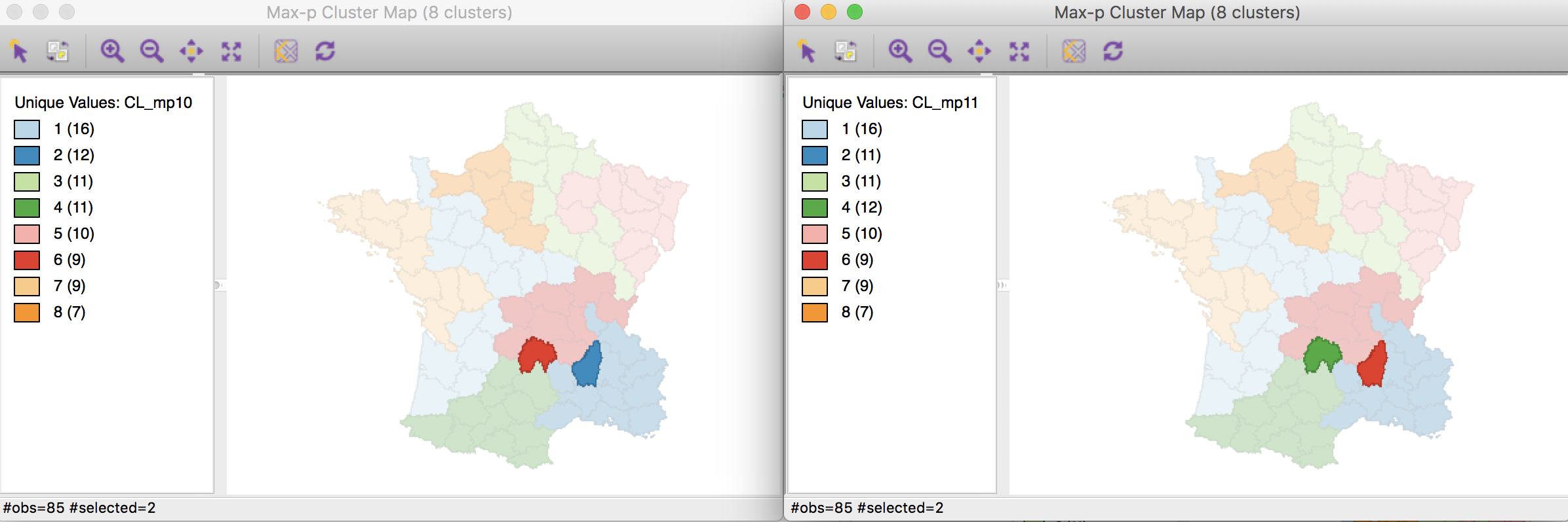
Max-p cluster map comparisons
The summary characteristics turn out to be very similar to the previous solution, but with a slightly better value for the ratio objective, which now is 0.526.
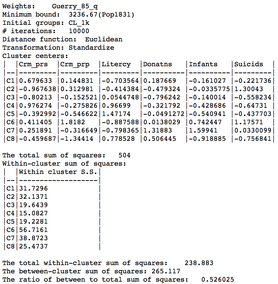
Max-p cluster summary, 10000 iterations after CL1
In practice, further experimentation with initial starting values and the number of iterations should be carried out to ensure that the solution is stable.
Summary
Finally, we run each method using k=8 to allow for comparison with max-p, and summarize the value of the objective function in the table below. In this particular example, the max-p method obtains the solution that is closest to the unconstrained K-means.
| Method | Ratio |
|---|---|
| K-Means | 0.627 |
| K-Means (centroids) | 0.632 |
| K-Means weighted 1.0 | 0.357 |
| K-Means weighted 0.89 | 0.429 |
| Skater | 0.496 |
| Max-p | 0.526 |
References
Assuncao, Renato, M Neves, G Camara, and C Da Costa Freitas. 2006. “Efficient Regionalization Techniques for Socio-Economic Geographical Units Using Minimum Spanning Trees.” International Journal of Geographical Information Science 20: 797–811.
Duque, Juan C., Luc Anselin, and Sergio J. Rey. 2012. “The Max-P Regions Problem.” Journal of Regional Science 52: 397–419.
Haining, R, S Wise, and J Ma. 2000. “Designing and Implementing Software for Spatial Statistical Analysis in a GIS Environment.” Journal of Geographical Systems 2: 257–86.
-
University of Chicago, Center for Spatial Data Science – anselin@uchicago.edu↩
-
For detailed instructions, see the previous chapter.↩