Spatial Clustering (3)
Spatially Constrained Clustering - Partitioning Methods
Luc Anselin1
12/07/2020 (latest update)
Introduction
In this chapter, we continue the treatment of clustering methods where the spatial constraint is imposed explicitly. However, in contrast to the previous chapter, where hierarchical approaches were covered, we now consider partitioning methods. In the literature, this is often referred to as the p-regions problem, i.e., a problem of combining n spatial units into p larger regions that are made up of contiguous entities and maximize internal homogeneity.
A discussion of the general issues and extensive literature reviews can be found in Duque, Ramos, and Suriñach (2007), Duque, Church, and Middleton (2011), and Li, Church, and Goodchild (2014), among others. Here, we focus our attention on two approaches. One is the automatic zoning problem or AZP, originally considered by Openshaw (1977) (later, AZP is also referred to as the automatic zoning procedure). As in the methods discussed previously, this requires a prior specification of the number of zones or regions (p).2
In contrast, in the so-called max-p regions model, proposed in Duque, Anselin, and Rey (2012), the number of regions becomes endogenous, and heuristics are developed to find the allocation of spatial units into the largest number of regions (max-p), such that a spatially extensive minimum threshold condition is met.
We continue to use the Guerry sample data set to illustrate these approaches and the small Arizona county example to show the detailed steps in the algorithms.
Objectives
-
Understand the logic behind the automatic zoning procedure (AZP)
-
Appreciate the differences between greedy, simulated annealing and tabu searches
-
Gain insight into the different ways to fine tune AZP using ARiSeL
-
Identify contiguous clusters with the number of clusters as endogenous with max-p
-
Understand the different stages of the max-p algorithm
-
Appreciate the sensitivity of the AZP and max-p heuristics to various tuning parameters
GeoDa functions covered
- Clusters > AZP
- select AZP method
- ARiSeL option
- set initial regions
- Clusters > Max-p
Preliminaries
We continue to use the Guerry data set and also need a spatial weights matrix in the form of queen contiguity.
Automatic Zoning Procedure (AZP)
Principle
The automatic zoning procedure (AZP) was initially outlined in Openshaw (1977) as a way to address some of the consequences of the modifiable areal unit problem (MAUP). In essence, it consists of a heuristic to find the best set of combinations of contiguous spatial units into p regions, minimizing the within sum of squares as a criterion of homogeneity. The number of regions needs to be specified beforehand, as in most other clustering methods considered so far.
The problem is NP-hard, so that it is impossible to find an analytical solution. Also, in all but toy problems, a full enumeration of all possible layouts is impractical. In Openshaw and Rao (1995), the original slow hill-climbing heuristic is augmented with a number of other approaches, such as simulated annealing and tabu search, to avoid the problem of being trapped in a local solution. None of the heuristics guarantee that a global solution is found, so sensitivity analysis and some experimentation with different starting points remains important.
Addressing the sensitivity of the solution to starting points is the motivation behind the automatic regionalization with initial seed location (ARiSeL) procedure, proposed by Duque and Church in 2004.3
It is important to keep in mind that just running AZP with the default settings is not sufficient. Several parameters need to be manipulated to get a good sense of what the best (or, a better) solution might be. This may seem a bit disconcerting at first, but it is intrinsic to the use of a heuristic that does not guarantee global optimality.
We now consider each of the heuristics in turn.
AZP heuristic
The original AZP heuristic is a local optimization procedure that cycles through a series of possible swaps between spatial units at the boundary of a set of regions. The process starts with an initial feasible solution, i.e., a grouping of n spatial units into p contiguous regions. This initial solution can be constructed in a number of different ways. It is critical that the initial solution satisfies the contiguity constraints. For example, this can be accomplished by growing a set of contiguous regions from p randomly selected seed units by adding neighboring locations until the contiguity constraint can no longer be met.4
This process yields an initial list of regions and an allocation of each spatial unit to one and only one of the regions. At this point, a random region from the list is selected and its set of neighboring spatial units considered one at a time for a move from their original region to the region under consideration. Such a move is only allowed if it does not break the contiguity constraint in the origin region. If it improves on the overall objective function, i.e., the total within sum of squares, then the move is carried out.
With a new unit added to the region under consideration, its neighbor structure (spatial weights) needs to be updated to include new neighbors from the spatial unit that was moved and that were not part of the original neighbor list.
The evaluation is continued and moves implemented until the (updated) neighbor list is exhausted.
Now, the process moves to the next randomly picked region from the region list and repeats the evaluation of all the neighbors. When the region list is empty (i.e., all initial regions have been evaluated), the whole operation is repeated with the current region list until the improvement in the objective function falls below a critical convergence criterion.
Note that the heuristic is local in that it does not try to find the globally best move. It considers only one neighbor of one region at a time, without checking on the potential swaps for the other neighbors or regions. As a result, the process can easily get trapped in a local optimum.
A detailed illustration of these steps is given in the Appendix.
Simulated annealing
The major idea behind methods to avoid being trapped in a local optimum amounts to allowing non-improving moves at one or more stages in the optimization process. This purposeful moving in the wrong direction provides a way to escape from potentially inferior local optima.
One method to accomplish this is so-called simulated annealing. This approach originated in physics , and is also known as the Metropolis algorithm, commonly used in Markov Chain Monte Carlo simulation (Metropolis et al. 1953). The idea is to introduce some randomness into the decision to accept a non-improving move, but to make such moves less and less likely as the heuristic proceeds.
If a move (i.e., a move of a spatial unit into a new region) does not improve the objective function, it can still be accepted with a probability based on the so-called Boltzmann equation. This compares the (negative) exponential of the relative change in the objective function to a 0-1 uniform random number. The exponent is divided by a factor, called the temperature, which is decreased (lowered) as the process goes on.
Formally, with \(\Delta O/O\) as the relative change in the objective
function and \(r\) as a draw from a
uniform 0-1 random distribution, the condition of acceptance of a non-improving move is:
\[ r < e^\frac{-\Delta O/O}{T(k)},\]
where \(T(k)\) is the temperature at annealing step k.5
Typically \(k\) is constrained so that only a limited number of such
annealing moves are allowed per iteration. In
addition, only a limited number of iterations are allowed (in GeoDa, this is controlled by the
maxit parameter).
The starting temperature is typically taken as \(T = 1\) and gradually
reduced at each annealing step \(k\)
by means of a cooling rate \(c\), such that:
\[T(k) = c.T(k-1).\]
In GeoDa, the default cooling rate is set to 0.85, but typically some experimentation may be
needed.6
The effect of the cooling rate is that \(T(k)\) becomes smaller, so that the value in the negative exponent becomes larger, which yields a smaller value of the result to compare to \(r\).7 Since the mean of the uniform 0-1 random draw \(r\) is 0.5, smaller and smaller values on the right-hand side of the Boltzmann equation will result is less and less likely acceptance of non-improving moves.
In AZP, the simulated annealing approach is applied to the evaluation step of the neighboring units, i.e., whether or not the move of a spatial unit from its origin region to the region under consideration will improve the objective.
In all other respects, simulated annealing AZP uses the same steps as outlined above for the original AZP heuristic.
Tabu search
The tabu search is yet another method designed to avoid getting trapped in a local optimum. It was originally suggested in the context of mixed integer programming by Glover (1977), but has found wide applicability in a range of combinatorial problems, including AZP (originally introduced in this context by Openshaw and Rao 1995).
One aspect of the local search in AZP is that there may be a lot of cycling, in the sense that spatial units are moved from one region to another and at a later step moved back to the original region. In order to avoid this, a tabu search maintains a so-called tabu list that contains a number of (return) steps that are prohibited.
With a given regional layout, all possible swaps are considered from a list of candidates
from the adjoining neighbors. Each of these neighbors that is not in the current tabu list is considered
for a possible swap, and the best swap is selected. If the best swap improves the overall objective
function (the total within sum of squares), then it is implemented and the reverse move is added to the
tabu list. In practice, this means that this move cannot be considered for \(R\) iterations, where \(R\) is the length
of the tabu list, or the Tabu Length parameter in GeoDa.
If the best swap does not improve the overall objective then the next available tabu move is considered (a so-called aspirational move). If the latter improves on the overall objective, it is carried out and the reverse move is added to the tabu list. If the aspirational move does not improve the objective, then the best swap is implemented anyway and its reverse move is also added to the tabu list. In a sense, rather than making no move, a move is made that makes the overall objective (slightly) worse. The number of such non-improving moves is limited by the ConvTabu parameter.
The tabu approach can dramatically improve the quality of the end result of the search. However, a critical parameter is the length of the tabu list, or, equivalently, the number of iterations that a tabu move cannot be considered. The results can be highly sensitive to the selection of this parameter, so that some experimentation is recommended (for examples, see the detailed experiments in Duque, Anselin, and Rey 2012).
ARiSeL
The ARiSeL approach, which stands for automatic regionalization with initial seed location, is an alternative way to select the initial feasible solution. In the original AZP formulation, this initial solution is based on a random choice of p seeds, and the initial feasible regions are grown around these seeds by adding the nearest neighbors. It turns out that the result of AZP is highly sensitive to this starting point.
Duque and Church proposed the ARiSeL alternative, based on seeds obtained from a Kmeans++ procedure.8 This yields better starting points for
growing a
whole collection of initial feasible regions. Then the best such solution is chosen as the basis
for a tabu search. In GeoDa, the ARiSeL approach is available as an option for all three search
heuristics.
Implementation
The AZP option is available from the cluster toolbar icon as the first item in the last group, as shown in Figure 1, or from the menu, as Clusters > AZP.
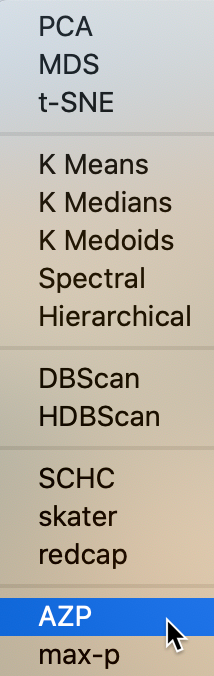
Figure 1: AZP cluster option
The AZP Settings interface takes the familiar form, shown in Figure 2. In addition to the variables, the number of clusters needs to be specified, and the method of interest selected: AZP (the default local search), AZP-Simulated Annealing, or AZP-Tabu Search. Other options are discussed below.
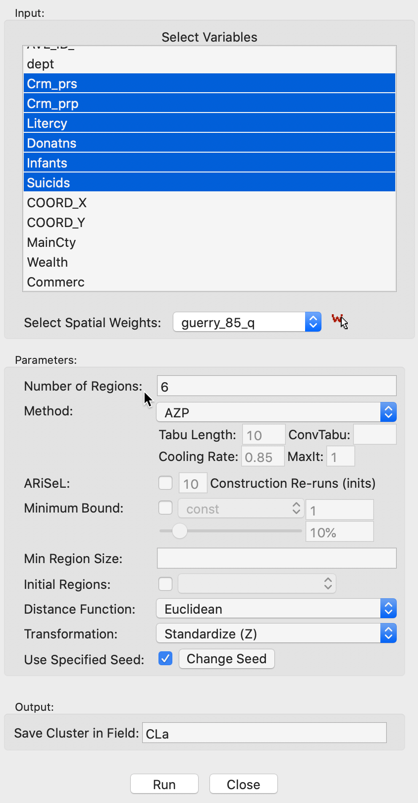
Figure 2: AZP Settings interface
We continue with the same example as before, using the Guerry sample data with queen contiguity spatial weights. The variables are again Crm_prs, Crm_prp, Litercy, Donatns, Infants, Suicids, used in standardized form. We set the number of regions to 6 and leave all the other defaults as specified.
As a frame of reference, we note that the unconstrained k-means results yielded a between to total sum of squares ratio of 0.552. From the previous chapter, we recall that the unconstrained hierarchical clusters best result for p=6 was 0.532. Among the spatially constrained techniques, we found the ratio to range from 0.420 for Skater to 0.462 for SCHC with Ward’s linkage, with Redcap Full-Order-Ward close at 0.460.
Local search
The default result is shown in Figure 3, with the Method option set to AZP. We have three fairly equally balanced regions (27, 25 and 18), and three smaller ones (7, 4, 4). The regions are less compact than in the last chapter, with some string-like chains, as in region 6. The between to total sum of squares ratio is 0.431, better than skater, but not as good as SCHC or Redcap with Ward’s linkage.
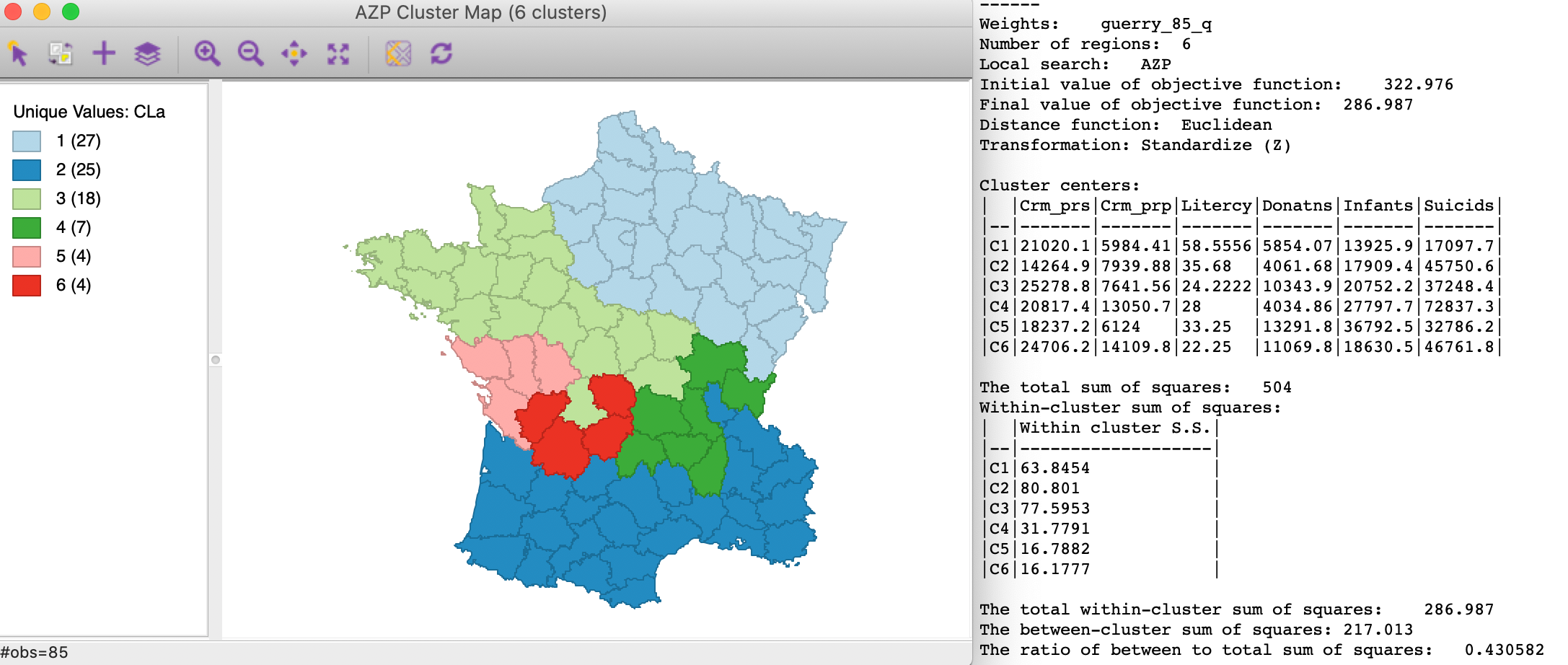
Figure 3: AZP local search clusters
Simulated annealing
When the simulated annealing option is selected from the Method drop-down list, with the default cooling rate of 0.85, the result is improved, but only slightly. As shown in Figure 4, the resulting clusters take on a very different shape compared to the local search result. The between to total sum of squares ratio is now 0.433.
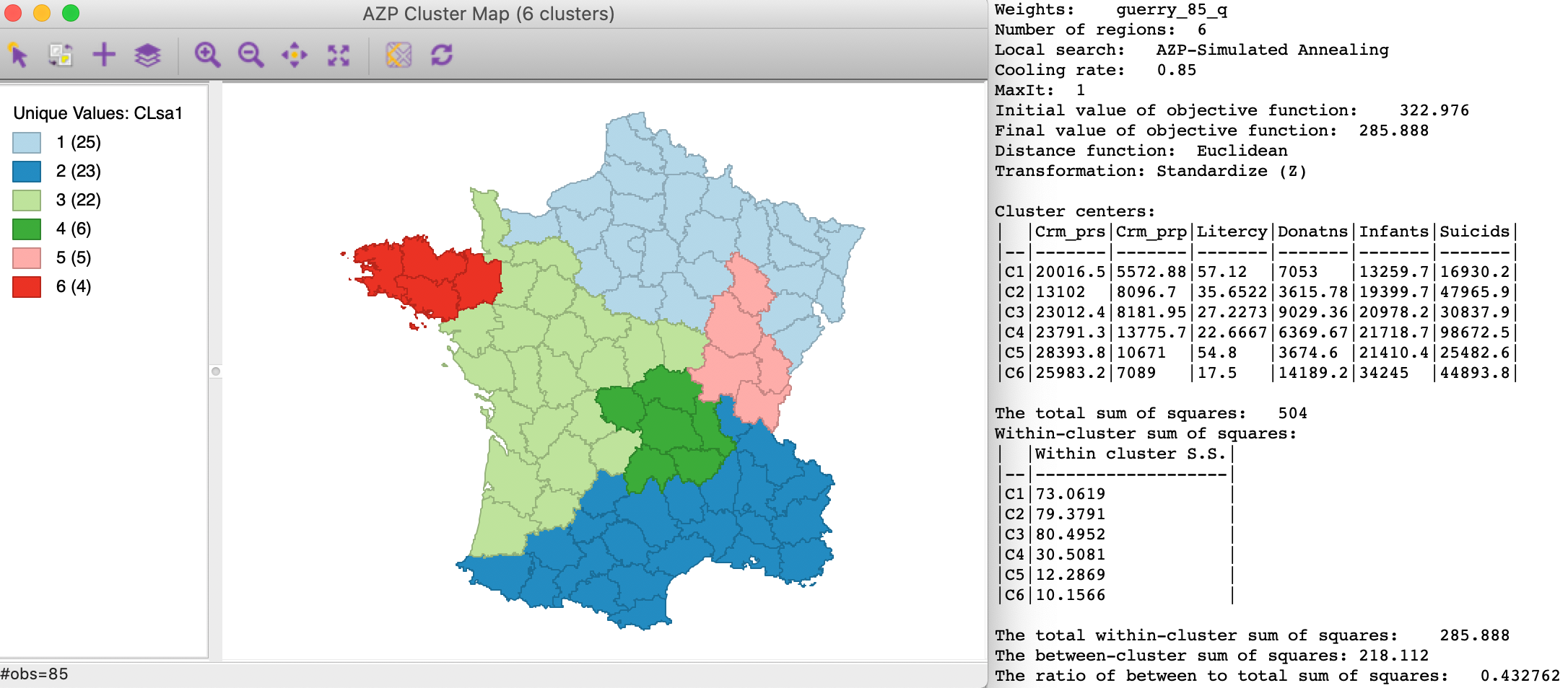
Figure 4: AZP simulated annealing clusters - cooling rate=0.85
As mentioned, some experimentation with the cooling rate is important. In our example, setting the cooling rate to 0.9 yields a worse result (not shown), but a value of 0.80 gives the best result so far, shown in Figure 5. The between to total SS ratio is now 0.478, better than even the best result obtained with the hierarchical methods. Again, the clusters take on a totally different shape.
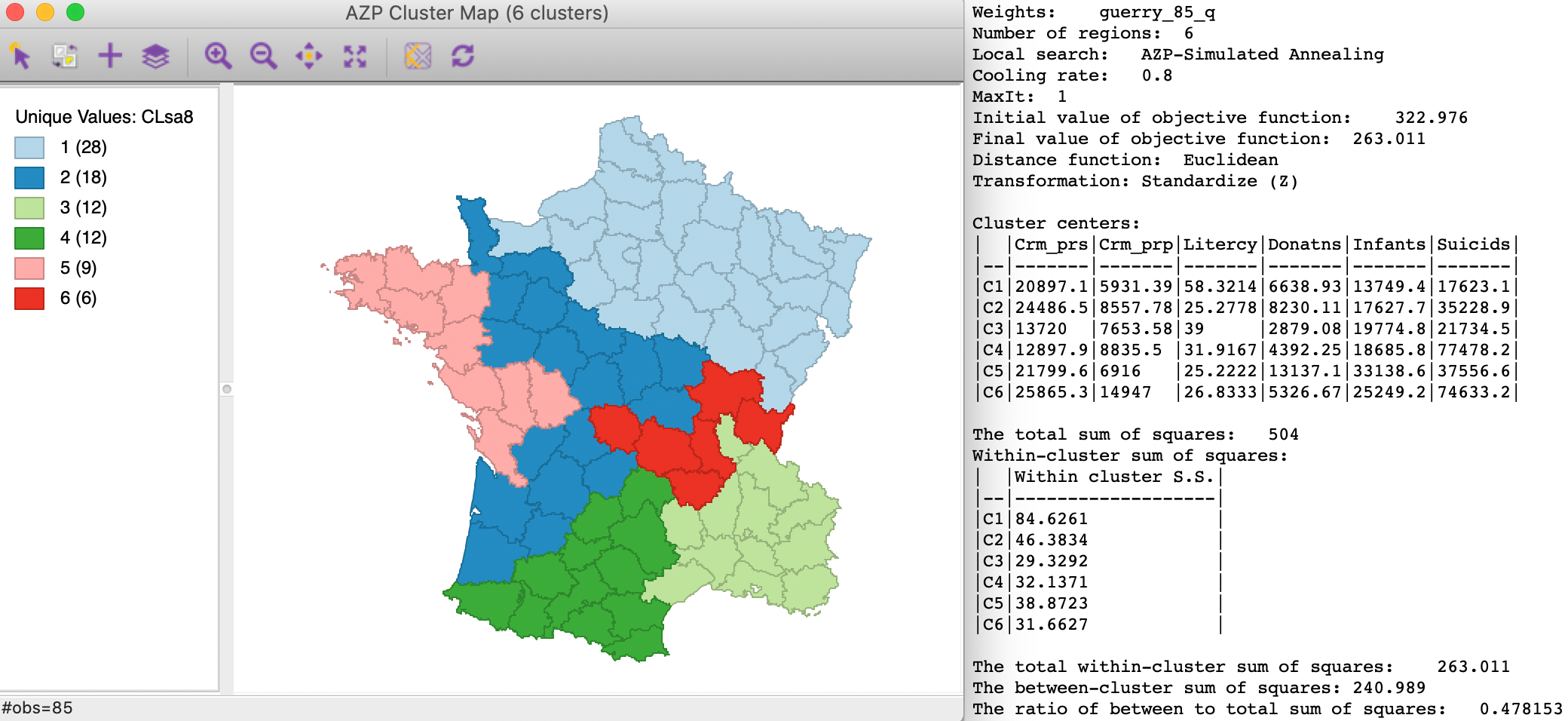
Figure 5: AZP simulated annealing clusters - cooling rate=0.80
Tabu search
The third option in the Method list is Tabu search. It is driven by two important parameters, the Tabu Length and ConvTabu, the number of non-improving moves that is allowed at each iteration. The default Tabu Length is 10 and ConvTabu is set to the maximum of 10 and \(n/p\). In our Guerry example with 85 observations and 6 regions, the default value for ConvTabu is thus 14. This is typically a good starting point, although it is by no means the only value that should be considered.
With the default settings, the results are as shown in Figure 6. This gives three fairly well balanced regions (27, 21 and 20), one roughly half this size (11), and two small ones (3 each). The between to total sum of squares ratio is 0.433, the same as the default result for simulated annealing.
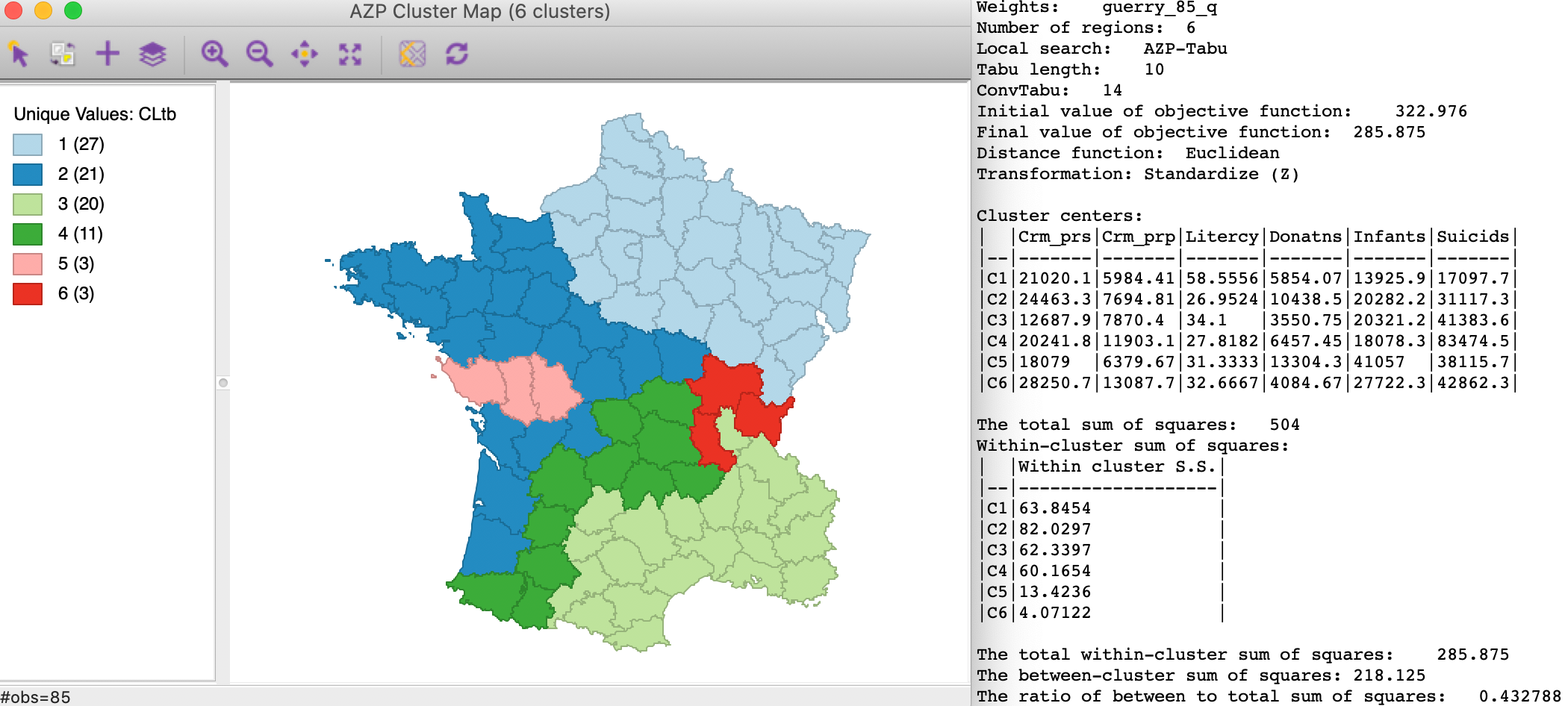
Figure 6: AZP tabu search - Tabu Length 10
Some experimentation with tabu length and convtabu can yield better results. For example, with the tabu length at 50 and convtabu at 25, we obtain a between to total ratio of 0.467, as in Figure 7. This is quite an improvement, but not as good as the best value for simulated annealing. Of course, it is possible that other combinations of these parameters give rise to even better results.
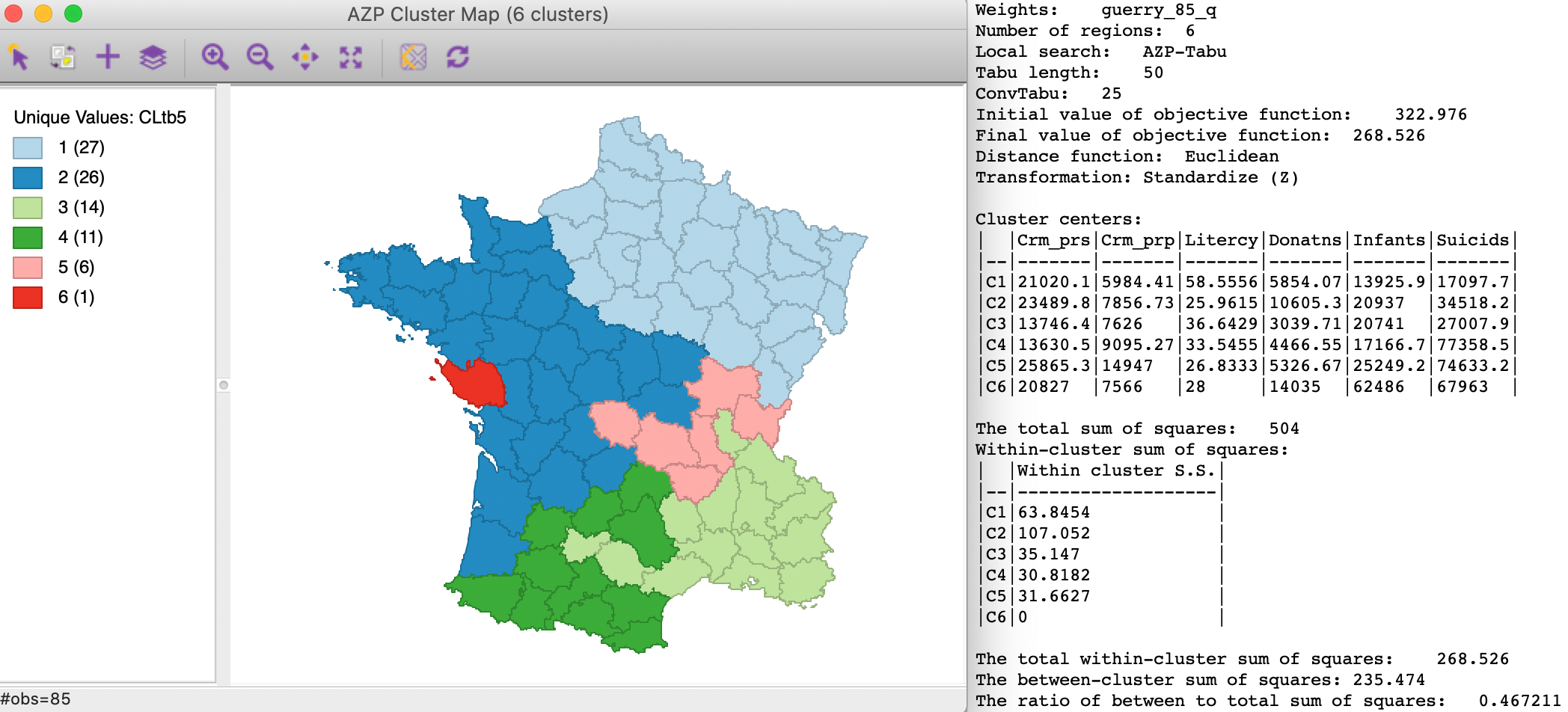
Figure 7: AZP tabu search - Tabu Length 50, ConvTabu 25
ARiSeL
The first stage in any of the AZP heuristics discussed so far is the construction of a feasible initial solution. In the classic approach, this is based on p random seeds from which feasible, i.e., contiguous, regions are grown. As the summary information on the results so far indicates, all solutions start with an Initial value of objective function of 322.976. In the ARiSeL approach, a (large) number of initial regions are generated, using the same logic for seeds as the kmeans++ approach. The best solution is selected as the new starting point. As long as the same random seed is used (see also below), the end point for an equal number of re-runs will be the same.
The ARiSeL approach is selected by checking the associated box and specifying the number of Construction Re-runs (see Figure 2). The default is 10 runs, but other values should definitely be considered. ARiSeL initiation can be combined with any of the three methods.
For example, consider the results in Figure 8, where 150 runs were used with the standard AZP heuristic. The initial value of the objective function is now quite a bit lower, at 284.942. In other words, the ARiSeL repeated runs yielded a feasible initial solution with a better value for the overall objective.
Once the new initial solution is determined, the heuristic works in exactly the same way as before. For standard AZP, this yields a between to total ratio of 0.436, only slightly better than the result based on a single random run, even though the starting point was much better.
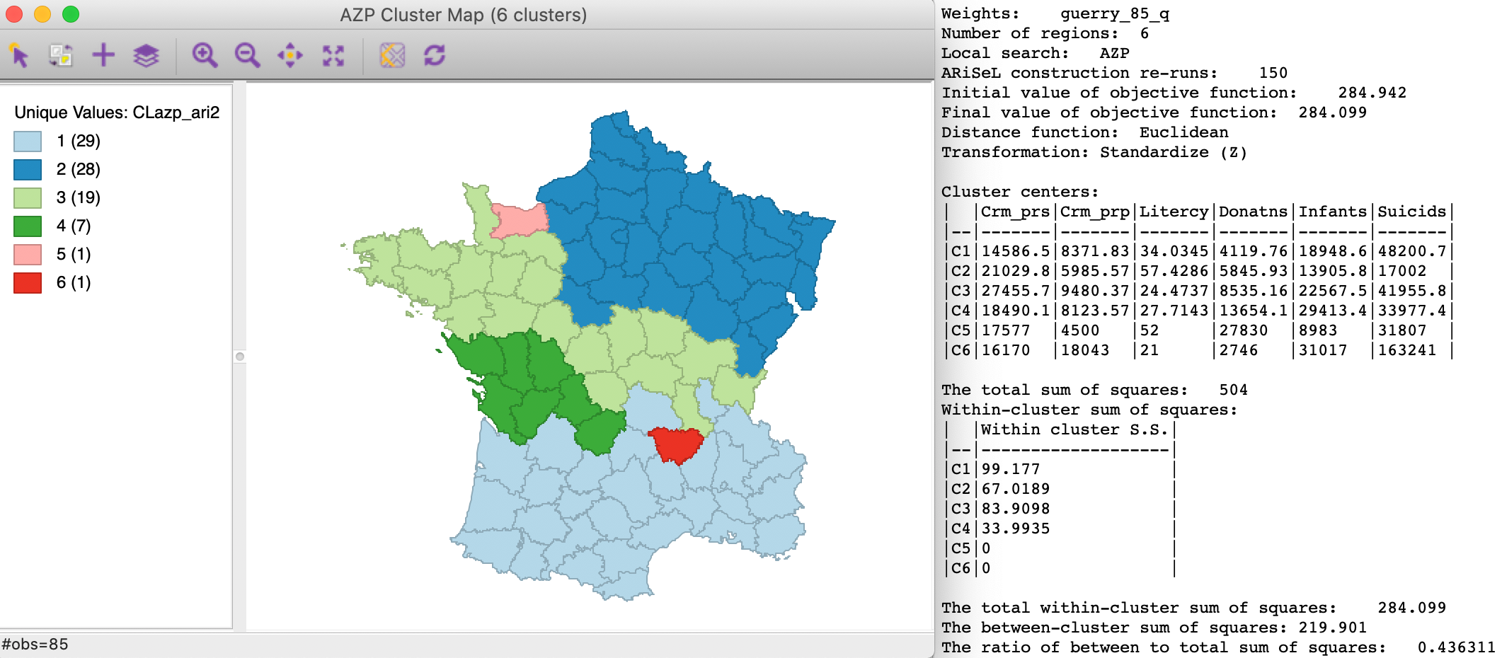
Figure 8: AZP with ARiSeL - 150 runs
Using 150 ARiSeL runs for the simulated annealing option (with a cooling rate of 0.8) does not improve on the previous result. As shown in Figure 9, the ultimate between to total ratio is 0.468, not as good as the 0.478 we obtained in Figure 5.
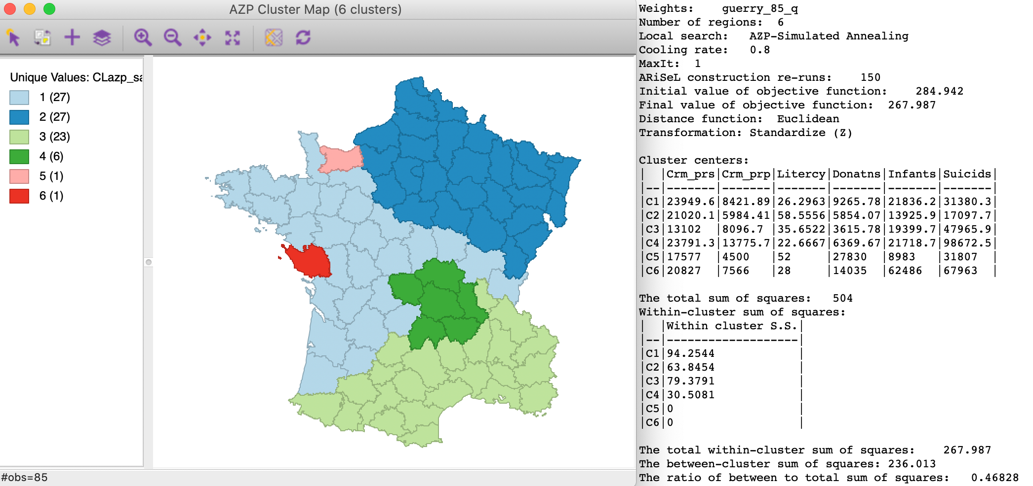
Figure 9: AZP Simulated Anealing with ARiSeL, cooling rate 0.80 - 150 runs
Finally, AZP-tabu with 150 ARiSeL runs also ends up with a worse result than before. As shown in Figure 10, the between to total ratio is 0.448, compared to 0.467 earlier.
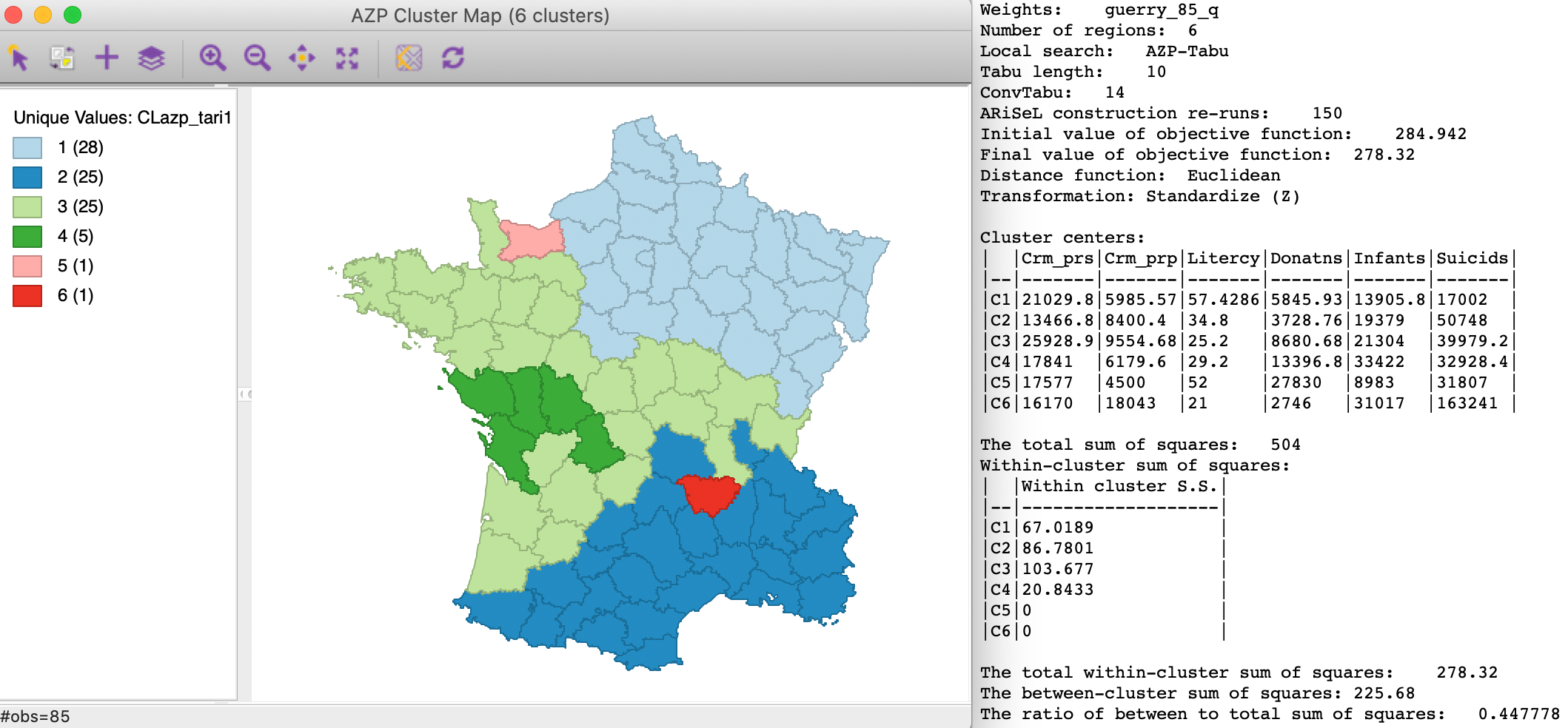
Figure 10: AZP tabu with ARiSeL, Tabu Length 10 - 150 runs
The main contribution of the ARiSeL approach is to yield better starting points for the respective heuristics. However, as we have seen in the illustrations given here, this does not always lead to better end results. Experimentation with other combinations of the various tuning parameter is needed to obtain a more complete picture of the various tradeoffs.
Changing the random seed
An alternative to the ARiSeL collection of starting runs is to change the random seed used to create the single feasible initial solution. In a sense, this changes the randomness of the starting seeds, but doesn’t guarantee any improvement. Also, once the Change Seed box is unchecked (see Figure 2), we lose the capacity to reproduce the various analyses. Preferably, we can change the seed to a specific value.
For example, we can turn the initial default seed of 123456789 to 12345678. This simple change has a major impact on the results, as shown in Figure 11. Even though the initial value of the objective function is worse than before, at 348.713, the ultimate result turns out to be better. In our example, for the standard AZP, this yields a between to total ratio of 0.450, much better than the result in Figure 3 for the original random seed (0.430), and even better than AZP-ARiSeL with the previous seed (0.436).
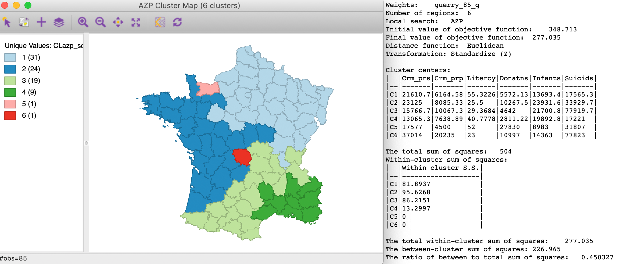
Figure 11: AZP with different random seed
In general, it is a good idea to include experiments with different random seeds in the range of sensitivity analyses.
To proceed, we return the initial seed to its default value of 123456789.
Initial regions
A different use of the various AZP heuristics is to potentially improve on solutions found by other methods. As we saw in the previous chapter, the hierarchical methods can be trapped into sub-optima, in that once a cut is made in the relevant spanning tree, it is impossible to move a spatial unit to a different branch.
Swapping units between regions is the essence of the heuristics behind the partitioning methods. An attempt to improve on one of the hierarchical solutions can be made by checking the Initial Regions box in the dialog shown in Figure 2. Next, a cluster classification variable must be selected from the drop-down list in order to initialize the process. This cluster variable was created in the Save Cluster in Field option during the relevant reference cluster exercise.
Here, we illustrate this by taking the final result from the skater algorithm with p=6. From the summary of this analysis (not shown here), we know that the final within sum of squares was 292.551 with a between to total ratio of 0.420. We use this as the initial feasible solution to the standard AZP heuristic, shown in Figure 12. The initial value of the objective function matches the end result of skater, as expected. The end result yields a between to total ratio of 0.463, a considerable improvement on the original skater regions.
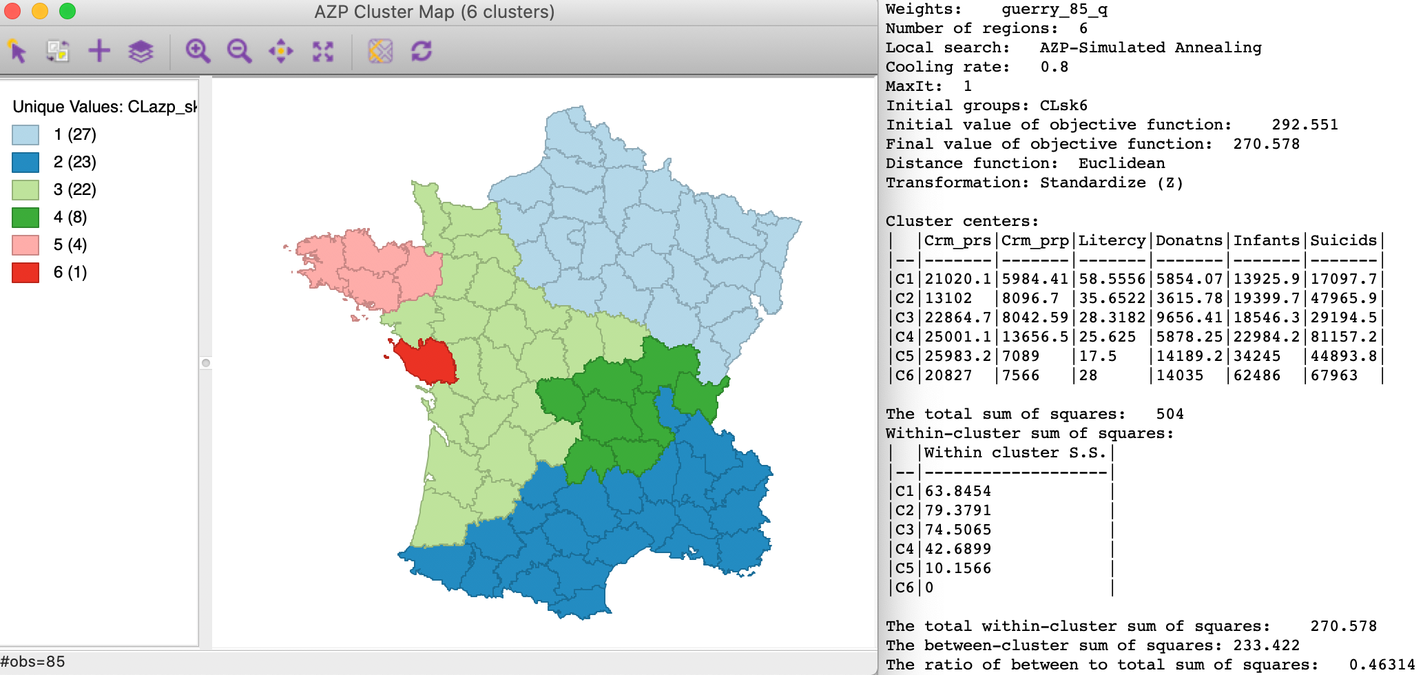
Figure 12: AZP Simulated Annealing with skater initial regions
As long as they satisfy the contiguity constraint, the Initial Region option can be used for other initial solutions as well, not just the results of previous clustering exercises.
Minimum bound
A final option is to set a Minimum Bound for each region in terms of a spatially extensive variable (such as population), or, alternatively, a Min Region Size (see Figure 2). This works in the same way as before, except that the contiguity constraint needs to be satisfied.
The initial feasible region must meet both the minimum bound as well as contiguity. After this, the same heuristics are applied. For example, in Figure 13, the results are shown for the default 10 % bound on Pop1831 (3236.67), using simulated annealing with a cooling rate of 0.80.
The smallest region contains 7 spatial units, which is more than for any of the unconstrained solutions. However, the other regions tend to be smaller, without a dominating entity as was often the case before. The initial value of the objective function (i.e., the starting point) is 359.154, larger than for any of the previous solutions. The between to total sum of squares ratio is 0.442, not as good as the unconstrained simulated annealing result (0.478). The decrease in internal homogeneity is the price to pay for imposing the minimum bound constraint.
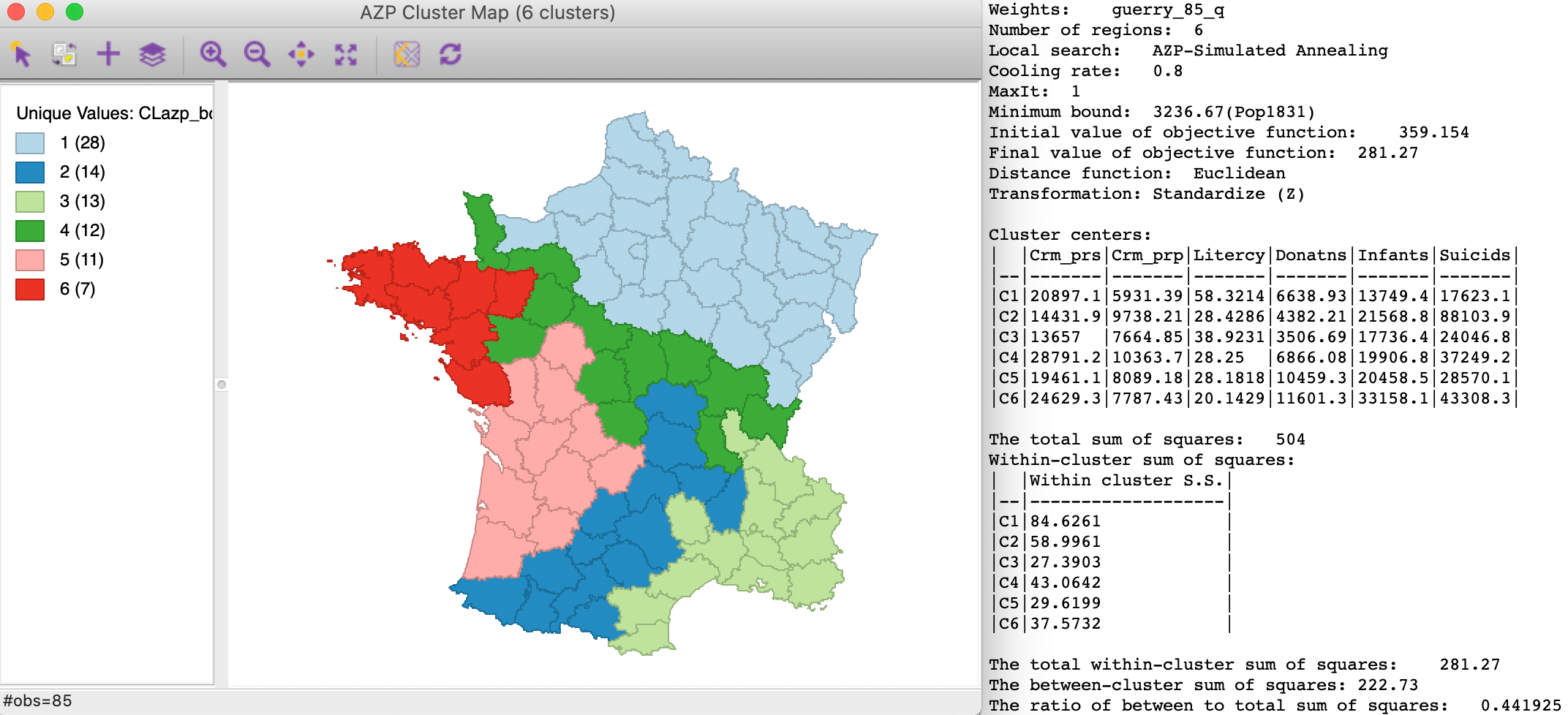
Figure 13: AZP Simulated Annealing with minimum bounds
Max-P Region Problem
Principle
The max-p region problem, outlined in Duque, Anselin, and Rey (2012), makes the number of regions (p) part of the solution process. This is accomplished by introducing a minimum size constraint for each cluster. In contrast to the use of such a constraint in earlier methods, where this was optional, for max-p the constraint is required. The size constraint is either a minimum value for a spatially extensive variable (such as population size, number of housing units), or a minimum number of spatial units that need to be contained in each region. Initially formulated as a standard regionalization problem, the method was extended to take into account a network structure in She, Duque, and Ye (2017).
In Duque, Anselin, and Rey (2012), the solution to the max-p region problem was presented as a special case of mixed integer programming (MIP), building on earlier approaches to incorporate contiguity constraints in site design problems given by Cova and Church (2000). Two key aspects are the formal incorporation of the contiguity constraint and the use of an objective function that combines the number of regions (p) and the overall homogeneity (minimizing the total with sum of squares). However, within this objective function, priority is given to finding a larger p rather than the maximum homogeneity. In contrast to an unconstrained problem, where a larger p will always yield a better measure of homogeneity (see the discussion of the elbow graph for k-means clustering), this is not the case when both a minimum size constraint and contiguity are imposed. In other words, simple minimization of the total within sum of squares may not necessarily yield the maximum p. Also, the maximum p solution may not give the best total within sum of squares. The tradeoff between the two sub-objectives is made explicit.
In a nutshell, the max-p algorithm will find the largest p that accommodates both the minimum size and contiguity constraints and then finds the regionalization for that value of p that yields the smallest total within sum of squares.
As it turns out, the formal MIP strategy becomes impractical for any but small size problems. Instead, a heuristic was proposed that consists of three important steps.9 As was the case for previous heuristics, this does not guarantee that a global optimum is found. Therefore, some experimentation with the various solution parameters is recommended. Even more than in the case of AZP, sensitivity analysis and the tuning of parameters is critical to find better solutions. Simply running the default will not be sufficient. The tradeoffs involved are complex and not always intuitive.
The specific steps in the max-p heuristic are considered next.
Max-p heuristic steps
The max-p heuristic outlined in Duque, Anselin, and Rey (2012) consists of three important phases: growth, assignment of enclaves, and spatial search.
The objective of the first phase is to find the largest possible value of p that accommodates both the minimum bounds and the contiguity constraints. In order to accomplish this, many different spatial layouts are grown by taking a random starting point and adding neighbors (and neighbors of neighbors) until the minimum bound is met. While it is practically impossible to consider all potential layouts, repeating this process for a large number of tries with different starting points will tend to yield a high value for p (if not the highest), given the constraints.
In the process of growing the layout, some spatial units will not be allocated to a region, when they and/or their neighbors do not meet the minimum bounds constraint or break the contiguity requirement. Such spatial units are stored in an enclave.
At the end of the growth process, we have one or more spatial layouts with p regions, where p is the largest value that could be obtained. Before we can proceed with the optimization process, we need to assign any spatial units contained in the enclave to an existing region, such that the overall within sum of squares is minimized. We illustrate this in our simple Arizona counties example in the Appendix.
Once that is accomplished, we take all feasible initial solutions for the given p and run them through the optimization process (in parallel). At this point, we proceed in exactly the same way as for AZP, using either greedy search, simulated annealing, or tabu search to find a (local) optimum. The best overall solution is chosen at the end.
Implementation
The max-p option is available from the main menu as Clusters > max-p, or as the last option from the Clusters toolbar icon, see Figure 1.
The variable settings dialog is again largely the same as for the other cluster algorithms. We select the same six variables as before, with the spatial weights as queen contiguity. In addition, we have to set the Mininum Bound variable and threshold. In our example, we again select Pop1831 and take the 10% default. Finally, we keep the number of Iterations at the default value of 99, as shown in Figure 14.
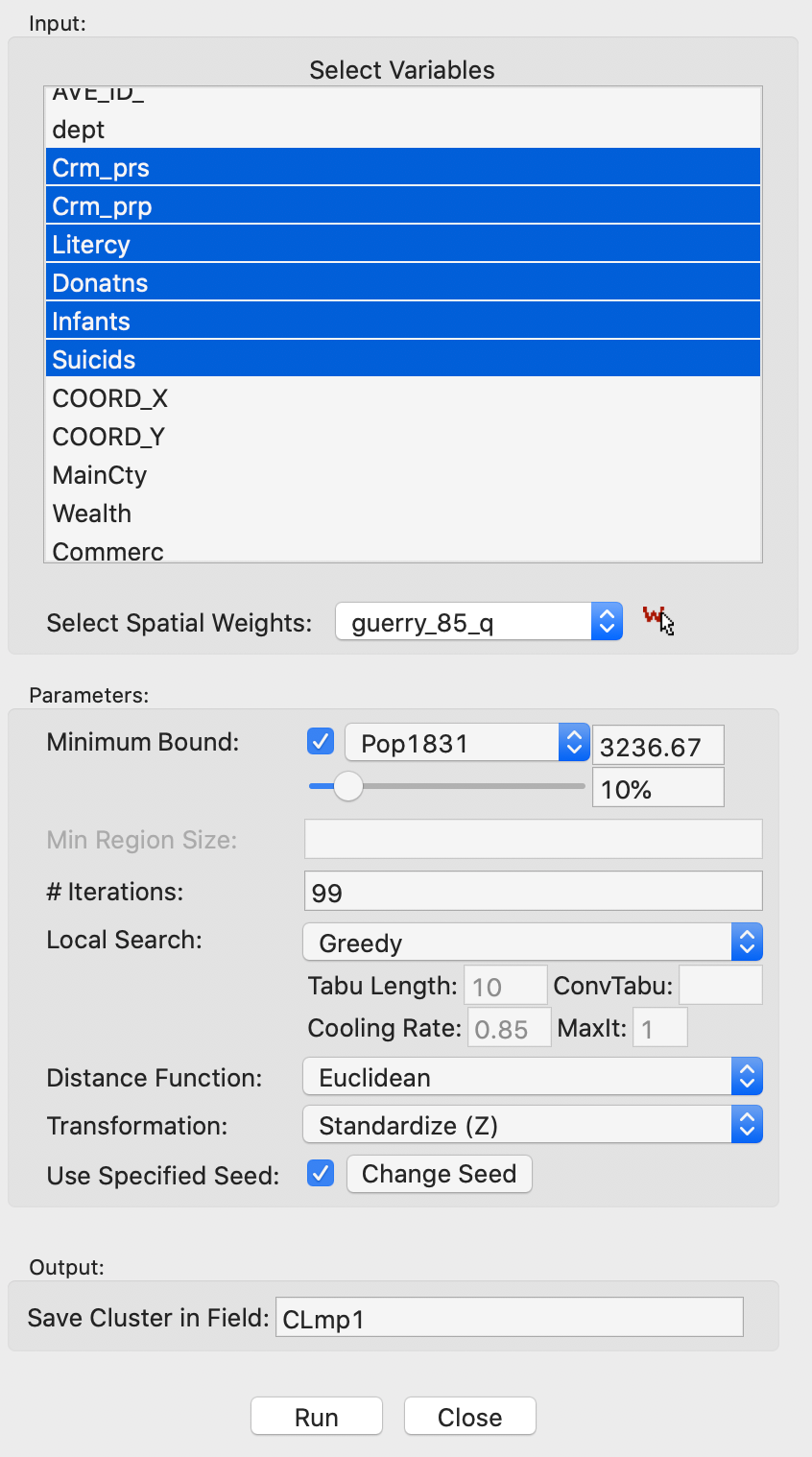
Figure 14: Max-p variables and parameter settings
Greedy
With all the settings to their default values, including 99 iterations, and with the original default random seed, the growth phase yields a maximum p value of 8.
The Greedy heuristic working from the collection of feasible initial solutions yields the regionalization shown in Figure 15. The clusters are well balanced and range in size from 8 to 17 spatial units. The between to total sum of squares ratio is 0.423. As a point of reference, we can compare this to the minimum bounds solution obtained by AZP for p=8 with the greedy algorithm, which yielded a ratio of 0.457 (not shown). At first sight, this result may be disappointing, but, as mentioned, further sensitivity analysis is in order.
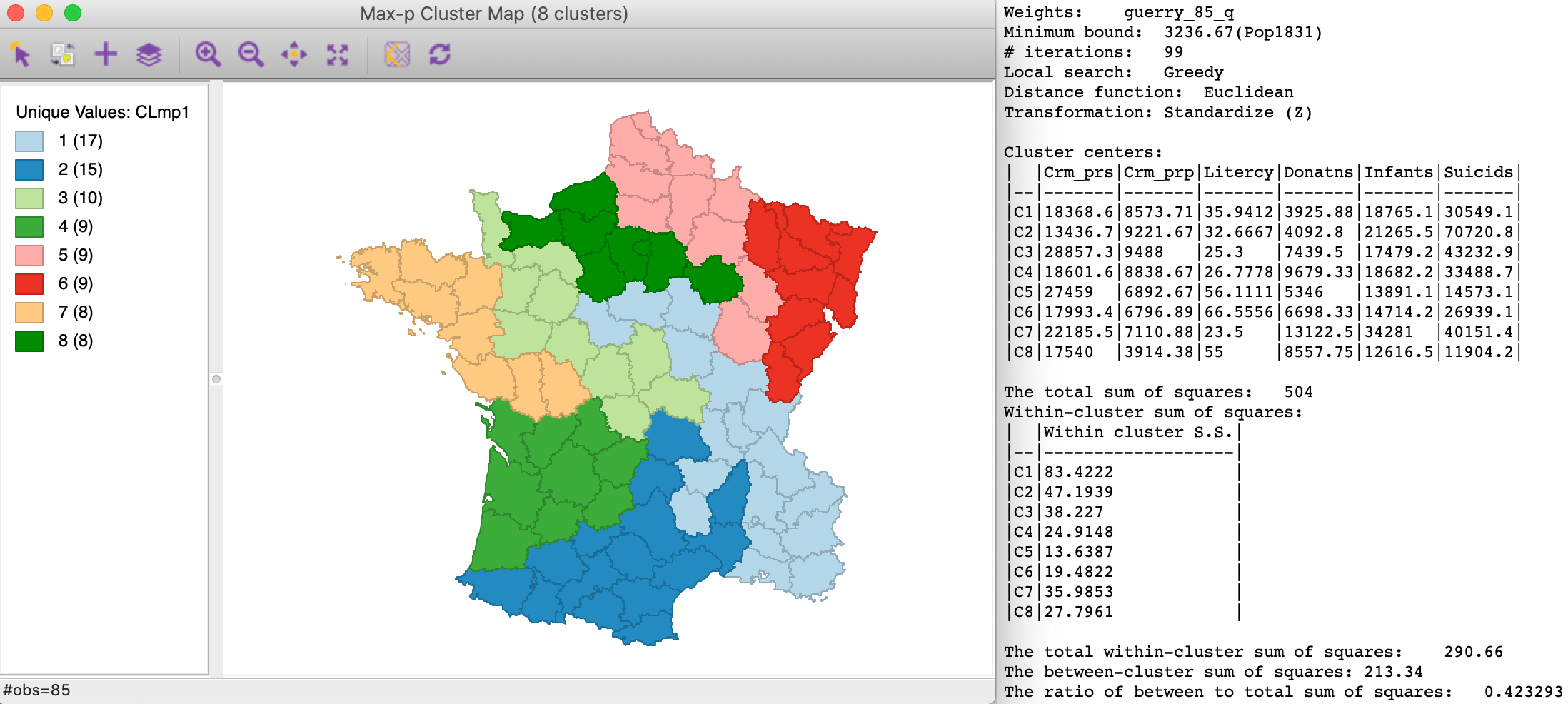
Figure 15: Max-p greedy heuristic - default settings
Simulated annealing
Again with the default settings, the Simulated Annealing method yields the results shown in Figure 16. Since the maximum value of p obtained is a function of the growth phase, this heuristic will start with the same set of feasible initial solutions as in the previous case. Only the final search phase is different.
The resulting layout shows some similarity in the northern and western regions with the regions in Figure 15, but the southern arrangement is quite different. The between to total ratio is 0.468, which again is worse than the outcome for AZP with p=8 and minimum bounds (0.480, not shown).
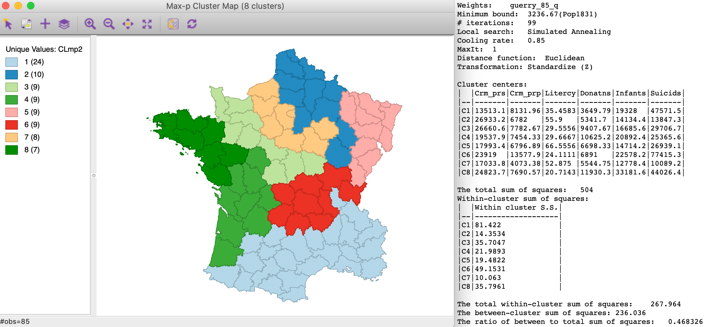
Figure 16: Max-p simulated annealing heuristic - default settings
Tabu search
Finally, Tabu Search starting from the same p=8 initial solutions yields the result shown in Figure 17. The layout is similar to the result for simulated annealing, with some re-arrangements among the northern clusters. In this instance, the between to total sum of squares ratio of 0.489 is actually better than the AZP minimum bound tabu search with p = 8 (0.476, not shown).
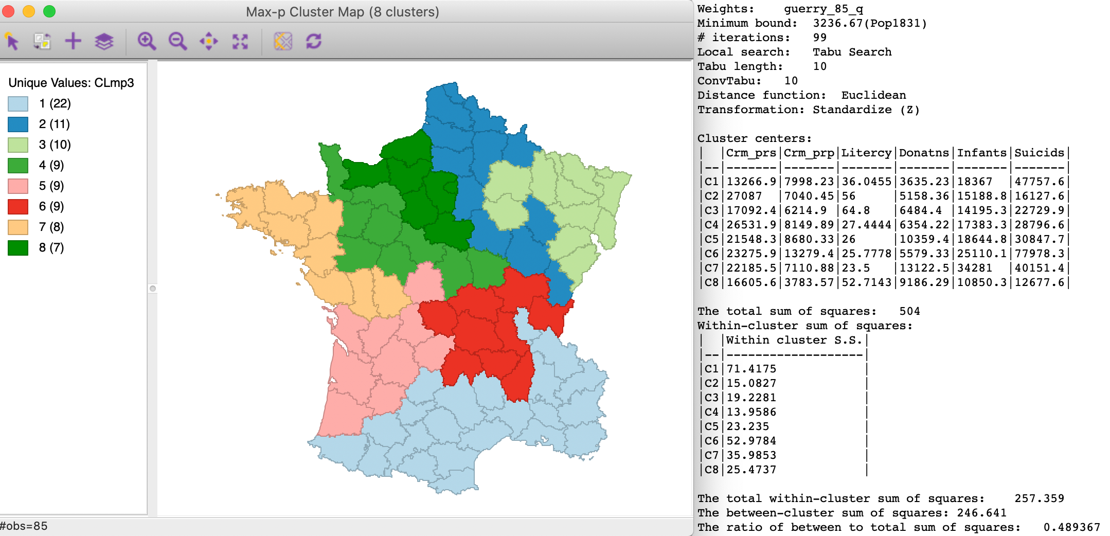
Figure 17: Max-p tabu heuristic - default settings
Sensitivity analysis
The max-p optimization algorithm is an iterative process, that moves from an initial feasible solution to a superior solution. However, this process may be slow and can get trapped in local optima. Hence, it behooves us to carry out an extensive sensitivity analysis.
There are two main aspects to this. One is to experiment with different parameters for the local search phase, which works in the same fashion as for AZP. The other is to increase the number of iterations for the growth phase, which can be critical in finding the highest value for p.
For example, increasing the number of iterations for the tabu search to 1000, with the same parameters as in Figure 17 yields a between to total ratio of 0.519, a considerable improvement from 0.489. The main reason for this is that the larger number of iterations provides a broader set of feasible initial solutions for p=8, from which the tabu heuristic can obtain a better final result.
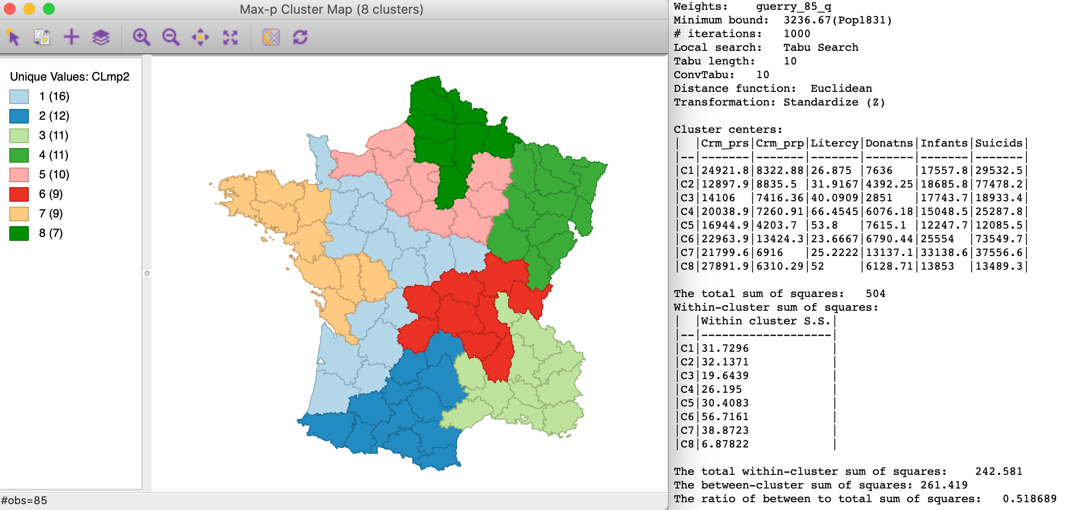
Figure 18: Max-p simulated annealing - 9999 iterations
A more dramatic illustration of the effect of the number of iterations is shown in Figure 19. With 9999 iterations to grow a feasible initial solution, the maximum p value obtained is now 9. Note that it turns out to be very difficult for the AZP routines to achieve a solution with p=9 that meets the minimum bound condition. Most attempts fail this criterion.10
Using a simulated annealing local search yields a between to total sum of squares ratio of 0.460.
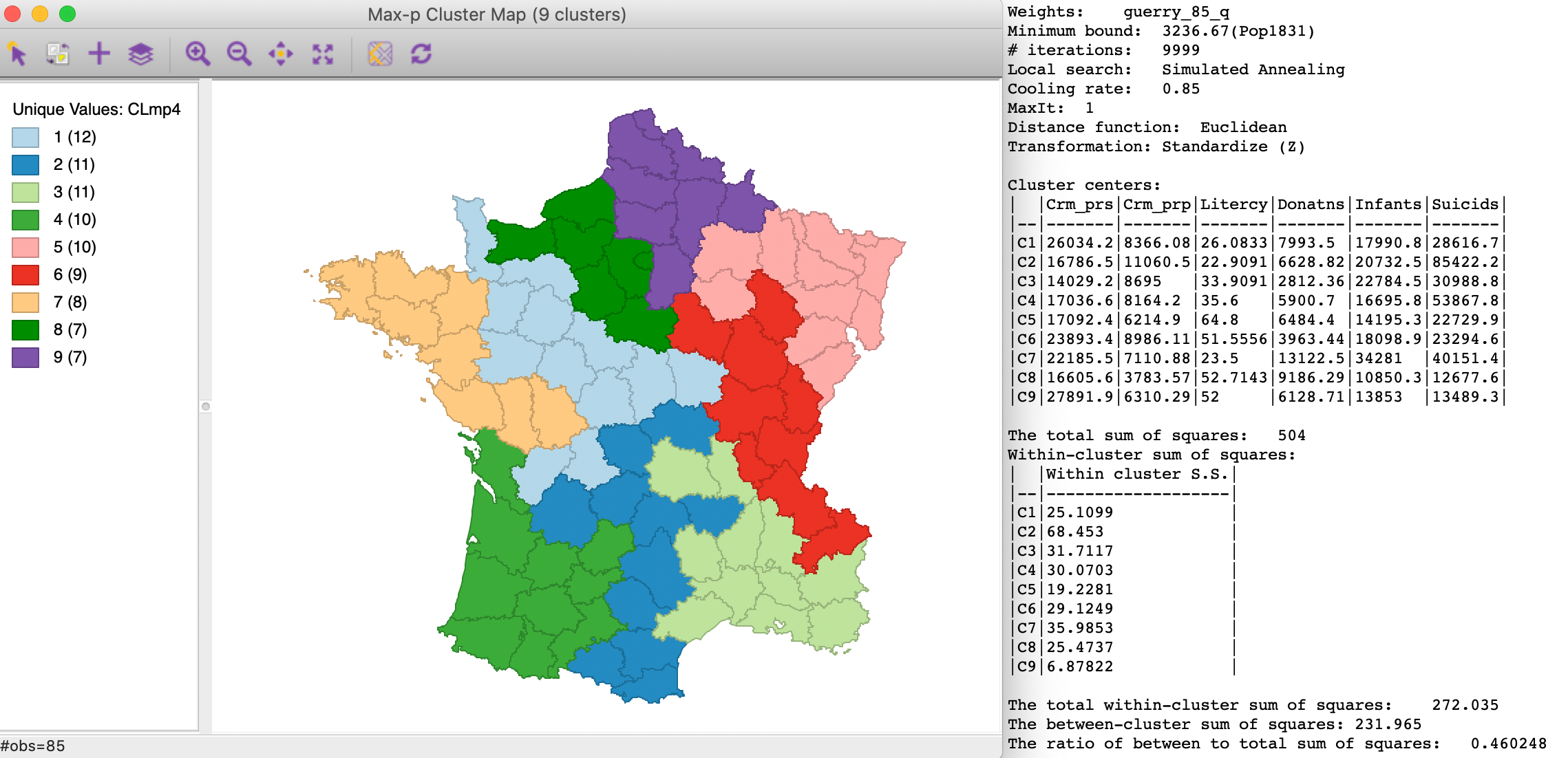
Figure 19: Max-p simulated annealing - 9999 iterations
Increasing the number of iterations somewhat obviates the need to fine tune the random number seed. Even though that is still possible, the effect of the initial seed diminishes as the number of iterations increases.
Optimizing parallel processing
A final optimization strategy consists of maximizing the number of cores utilized in parallel processing. This is important in the growth phase and the local search, both of which take advantage of parallel computing.
In machines with multiple cores, the number utlized by GeoDa can be set in the
Preferences panel, as shown
in Figure 20. The default is to manually specify a given number of cores.
However, by
unchecking the box, the program will determine internally the maximum available cores. With current
architectures
making 18 and more cores available, this has multiple advantages: it not only increases the speed of
computations,
but also allows larger problems to be solved and a wider range of initial feasible solutions to be
considered.
Specific results will depend on the available hardware.

Figure 20: Maximizing the number of cores for parallel processing
Appendix
Illustration of the AZP heuristic
We illustrate the logic behind the AZP greedy heuristic using the same example of Arizona counties as in the previous chapter. We again take the standardized value of the unemployment rate in 1990 as the single variable (SUE). In Figure 21, we show the data for each county and the associated squared value needed to compute the sum or squared deviations (SSD) for each cluster. As before, because the data are standardized, the starting total SSD is 13 (i.e., n - 1).
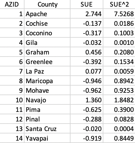
Figure 21: Arizona counties sample data
We start with a random initial feasible solution for k=4, depicted in Figure 22. We call the clusters a (7-9-14), b (1-3-10), c (4-8-11-12), and d (2-5-6-13). Since each cluster consists of contiguous units, it is a feasible solution.
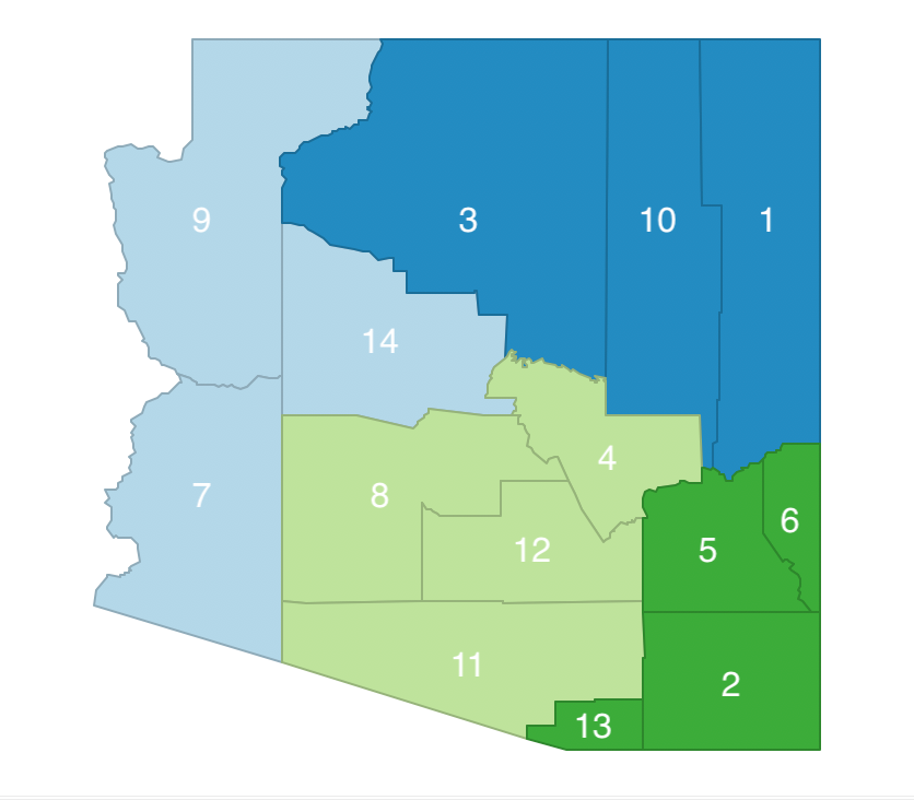
Figure 22: Arizona AZP initial feasible solution
The associated within sum of squares for each cluster is shown in Figure 23. The Total Within SSD for this layout is 6.2408.
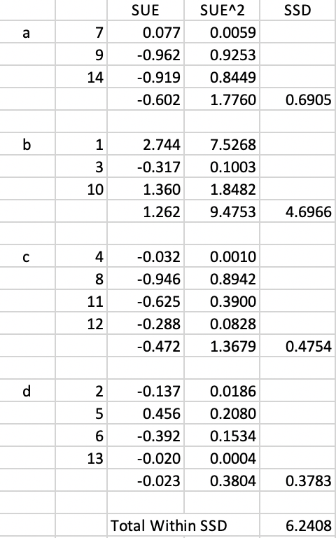
Figure 23: Arizona AZP initial Total Within SSD
Following the AZP logic, we construct a list of zones Z = [a, b, c, d]. We also make a list associating the proper cluster to each observation. In our example, this list is W = [b, d, b, c, d, d, a, c, a, b, c, c, d, a].
We randomly pick one of the zones, say c, and remove it from the list, so that now Z = [a, b, d]. We will continue to do this until the list is empty. Associated with cluster c is a list of its neighbors. These are highlighted in Figure 24. The list of neighbors is B = [2, 3, 5, 7, 10, 13, 14].
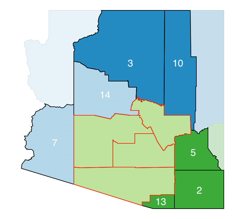
Figure 24: Arizona AZP initial neighbor list
We next randomly remove one of the elements of the neighbor list, say 2, and consider moving it from its current cluster (b) to cluster c. However, as shown in Figure 25, swapping observation 2 between b and c breaks the contiguity in cluster b (13 becomes an isolate), so this move is not allowed. As a result, 2 stays in cluster b for now.
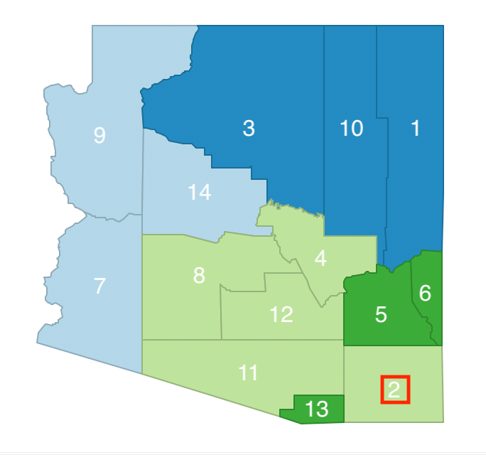
Figure 25: Arizona AZP step 1 neighbor selection - 2
We now randomly remove another element from the remaining list B = [3, 4, 5, 7, 10, 13, 14], say observation 14, and consider its move from cluster a to cluster c, as shown in Figure 26. This move does not break the contiguity between the remaining elements in cluster a (7 remains a neighbor of 9), so it is allowed.
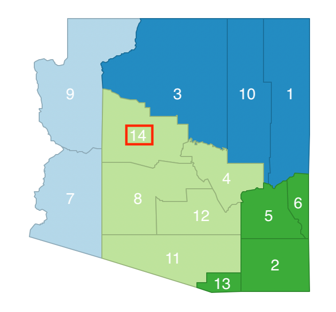
Figure 26: Arizona AZP step 2 neighbor selection - 14
As a result of this swap, cluster a now consists of 2 elements and cluster c of 5. The corresponding updated sums of squared deviations are given in Figure 27. The Total Within SSD becomes 6.2492, which is not an improvement over the current objective function (6.2408). As a consequence, this swap is rejected and 14 stays in cluster a.
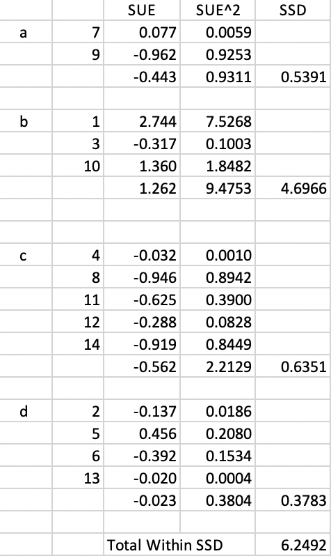
Figure 27: Arizona AZP step 2 Total Within SSD
The list of neighbors has now become B = [3, 4, 5, 7, 10, 13]. We randomly select 3 and consider its move from cluster b to cluster c, as in Figure 28. This move does not break the contiguity of the remaining elements in cluster b (10 and 1 remain neighbors), so it is allowed.
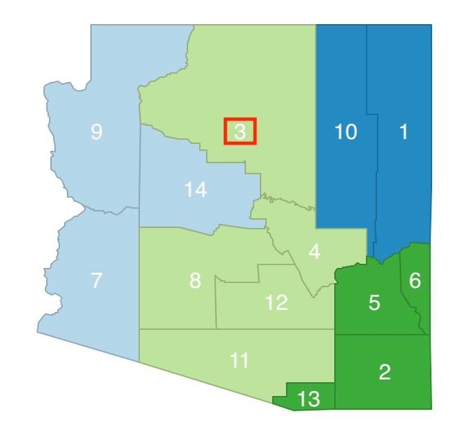
Figure 28: Arizona AZP step 3 neighbor selection - 3
At this point, cluster b has 2 elements and cluster c again 5. The associated SSD and Total Within SSD are listed in Figure 29. The swap of 3 from b to c yields an improvement in the overall objective from 6.2408 to 2.5213, so we keep the swap.
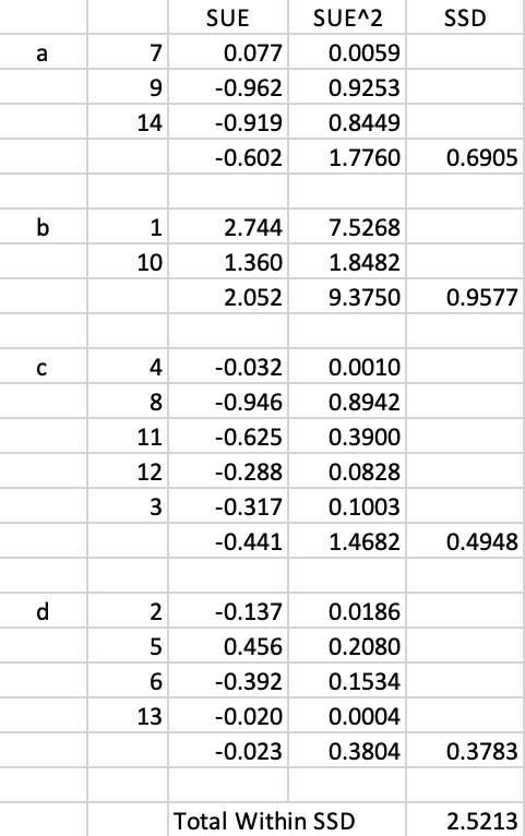
Figure 29: Arizona AZP step 3 Total Within SSD
We now need to re-evaluate the list of neighbors of the updated cluster c and add 9 as an additional neighbor to the list. The neighbor list thus becomes B = [4, 5, 7, 9, 10, 13].
The process continues by evaluating potential neighbor swaps until the list B is empty. At that point, we return to Z = [a, b, d] and randomly select another unit. We find its neighbor set and repeat the procedure until list Z is empty. At that point, we repeat the whole process for the updated list Z = [a, b, c, d] and continue this until convergence, i.e., until the improvement in the overall objective becomes less than a pre-specified threshold.
Illustration of the max-p heuristic
We illustrate the max-p heuristic continuing with the Arizona county example, now adding the population in 1990, i.e., PO90 as the minimum size constraint. Specifically, we impose a lower limit of a population size of 250,000. In Figure 30, the population counts for each of the counties is shown. The information relevant to assess the quality of the clusters was contained in Figure 21.
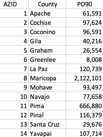
Figure 30: Arizona counties population
The heuristic consists of three phases. In the first, we grow feasible regions and establish the largest p that we can obtain. For those configurations that meet the max p, we assign the spatial units in the enclave to existing regions so as to minimize the total within sum of squares. Finally, we consider all those that meet the max p as feasible initial solutions for the optimization process.
We start the growth process by randomly selecting a location and determining its neighbors. In Figure 31, we chose 6 and find its three neighbors as 1, 5 and 2.
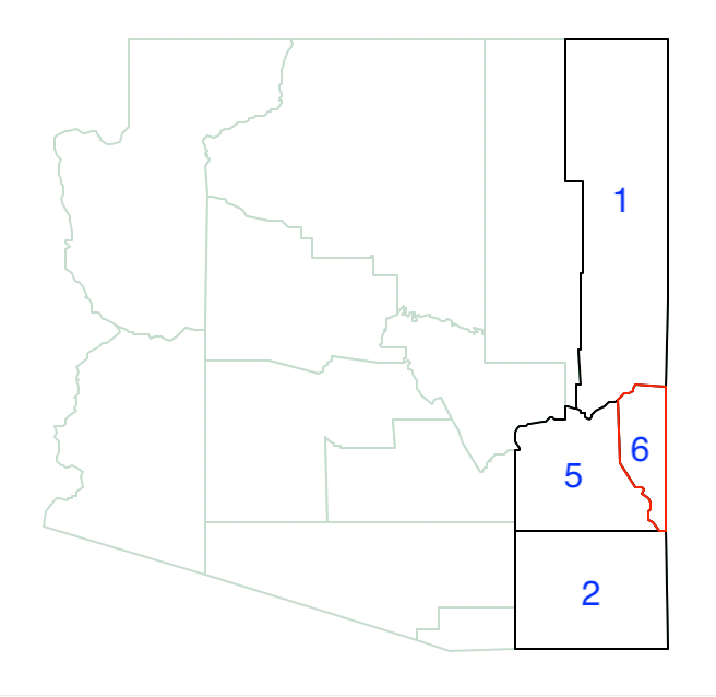
Figure 31: Arizona max-p grow start with 6
County 6 has a population of 8,008. We take the neighbor with the largest population - 2, with 97,624 - and join it with 6 to form the core of the first region. Its total population is 105,632, which does not meet the minimum threshold. At this point, we add the neighbors of 2 that are not already neighbors of 6.
As shown in Figure 32, the neighbor set now also includes 11 and 13.
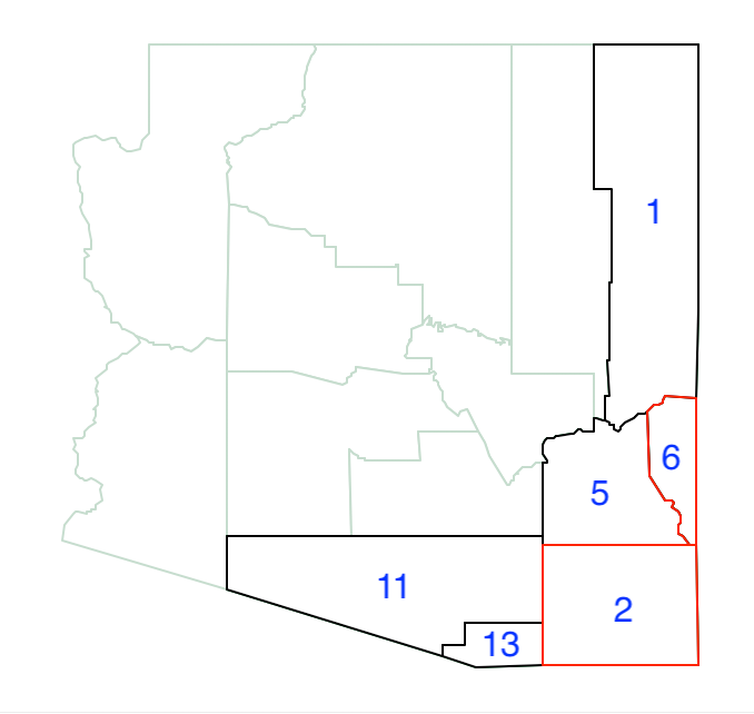
Figure 32: Arizona max-p grow - 6 and 2
Of the four neighbors, 11 has the largest population (666,880), which brings the total regional population to 764,504, well above the minimum bound. At this point, we create out first region as 6-2-11, shown in Figure 33.
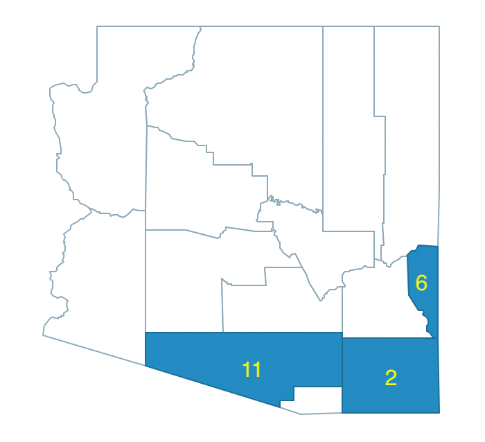
Figure 33: Arizona max-p grow - region 1
The second random seed turns out to be region 8. Its population is 2,122,101, well above the minimum bound. Therefore, it constitutes the second region in our growth process as a singleton, shown in Figure 34.
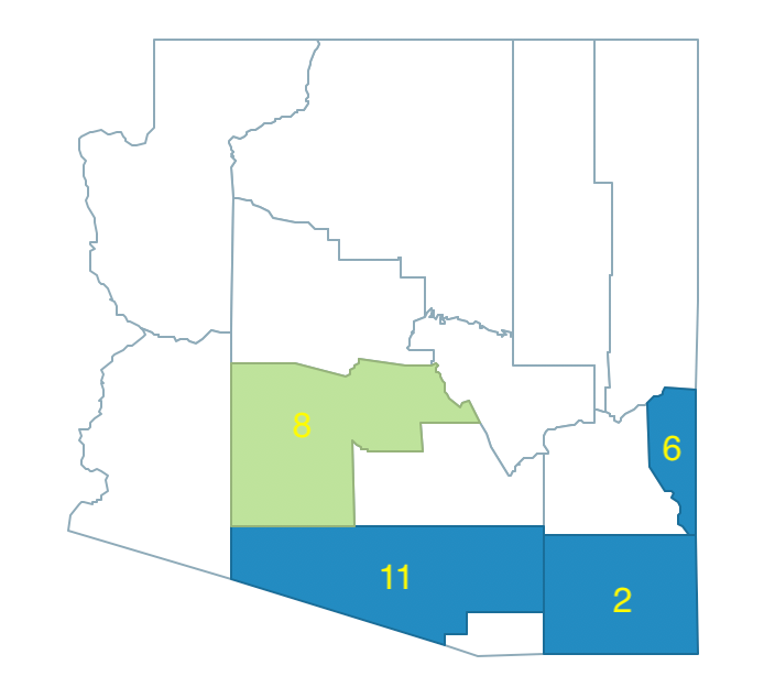
Figure 34: Arizona max-p grow - regions 1 and 2
The third random seed is 3, with neighbors 9, 14, 4 and 10, shown in Figure 35. The population of 3 is 96,591 and the largest neighbor is 14, with 107,714, for a total of 204,305, insufficient to meet the minimum bound.
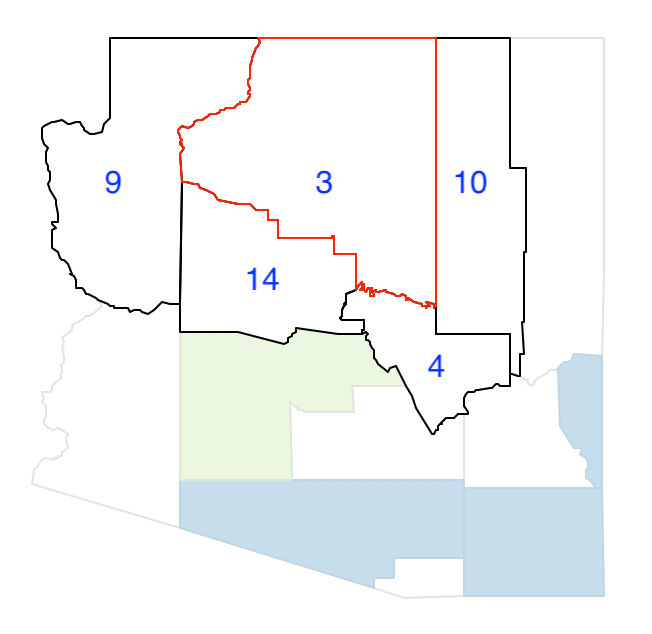
Figure 35: Arizona max-p grow - pick 3
Therefore, we group 3 and 14 and update the list of neighbors, shown in Figure 36. The only new neighbor is 7, since 8 is already part of a region.
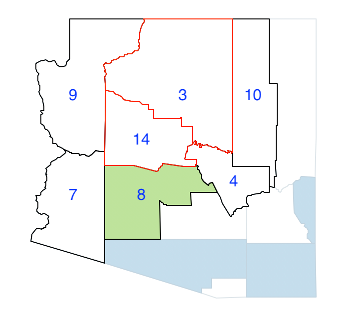
Figure 36: Arizona max-p grow - join 3 and 14
Since 7 has the largest population among the eligible neighbors (120,739) it is grouped with 3 and 14. This region meets the minimum threshold, with a total population of 325,044.
At this point, we have three regions, shown in Figure 37.
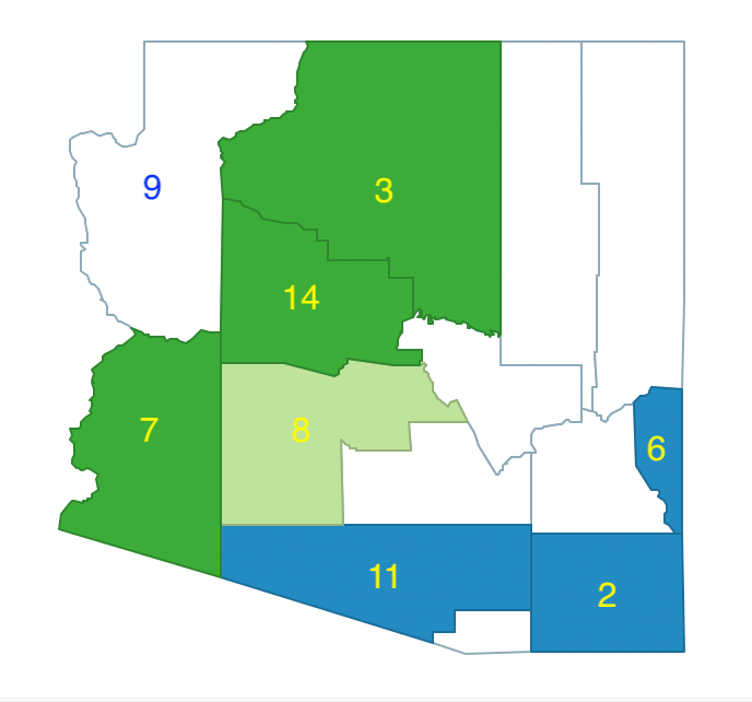
Figure 37: Arizona max-p grow - region 1, 2, 3
The next random seed is 9, with a population of 93,497. Its neighbors are already part of a previously part region (see Figure 37), so 9 cannot be turned into a region itself. Therefore it is relegated to the enclave.
The following random pick is 12, with a population of 116.379, and with neighbors 4, 8, 11 and 5 as shown in Figure 38. Of the neighbors, 8 and 11 are already part of other regions, so they cannot be considered.
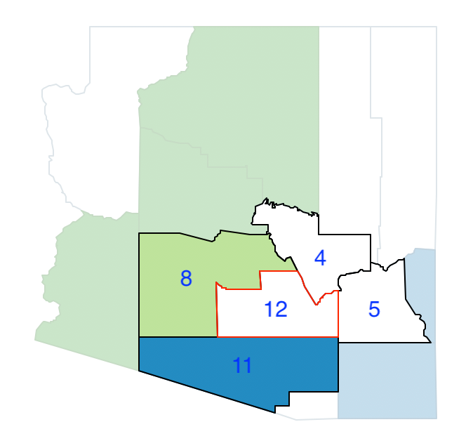
Figure 38: Arizona max-p grow - pick 12
Of the two neighbors of 12, 4 has the largest population, at 40,216, so it is joined with 12. However, their total population of 156,595 does not meet the threshold, so we need to consider the eligible neighbors of 4 as well. Of the six neighbors, only 10 is an addition, shown in Figure 39.
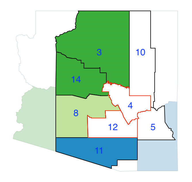
Figure 39: Arizona max-p grow - join 12 and 4
Between 5 and 10, the latter has the largest population (120,739), which brings the total for region 12-4-10 to 277,334. The new configuration with four regions is shown in Figure 40.
There are four remaining counties. We already have 9 in the enclave. Clearly, 13 with a population of 29,676 is not large enough to form a region by itself, so it is added to the enclave as well.
Similarly, the combination of 5 and 1 only yields a total of 88,145, which is insufficient to form a region, so they are both included in the enclave.
At this point, we have completed the growth phase and obtained p=4, with four counties left in the enclave, as in Figure 40. In a typical application, we would repeat this process many times and keep the solutions with the largest p. For those solutions, we need to establish the best feasible initial solution. To obtain this, we first need to complete the allocation process by assigning the elements in the enclave to one of the existing regions such as to minimize the total within sum of squares.
Figure 40: Arizona max-p enclaves - region 1, 2, 3, 4
In our example, for 9 and 13, the solution is straightforward: 9 is merged with 3-14-7, and 13 is merged with 11-2-6. For 5 and 1, the situation is a bit more complicated, since we could assign both to either cluster 1 (2-6-11-13) or cluster 4 (4-10-12), or one to each, for a total of four combinations.
The calculations of the respective sum of squared deviations are listed in Figure 41. The starting point is a total SSD between cluster 1 and 4 of 1.7899, at the top of the Figure. Next, we calculate the new SSD if 1 is added to the first cluster and 5 to the fourth, and vice versa. This increases the total SSD between the two clusters to respectively 9.1762 and 6.5476. Finally, we consider the scenarios where both 1 and 5 are added either to the first or to the fourth cluster. The results for the new SSD are, respectively, 9.1840 and 6.2903.
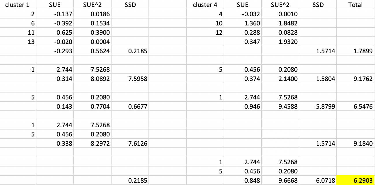
Figure 41: Arizona max-p assign enclaves
Consequently, the allocation that obtains the smallest within sum of squares is the regional configuration that assigns both 1 and 5 to region 4, shown in Figure 42. The constituting regions are 11-13-2-6, 8, 3-14-7-9, and 1-10-4-12-5.
At this point, we have a feasible initial solution that we can optimize by means of one of the three search algorithms, in the same fashion as for AZP.
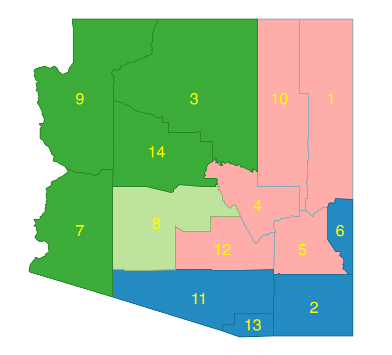
Figure 42: Arizona max-p - feasible initial regions
References
Cova, Thomas J., and Richard L. Church. 2000. “Contiguity Constraints for Single-Region Site Search Problems.” Geographical Analysis 32: 306–29.
Duque, Juan, Luc Anselin, and Sergio J. Rey. 2012. “The Max-P-Regions Problem.” Journal of Regional Science 52 (3): 397–419.
Duque, Juan Carlos, Raúl Ramos, and Jordi Suriñach. 2007. “Supervised Regionalization Methods: A Survey.” International Regional Science Review 30: 195–220.
Duque, Juan C., Richard L. Church, and Richard S. Middleton. 2011. “The P-Regions Problem.” Geographical Analysis 43: 104–26.
Glover, Fred. 1977. “Heuristics for Integer Programming Using Surrogate Constraints.” Decision Science 8: 156–66.
Laura, Jason, Wenwen Li, Sergio J. Rey, and Luc Anselin. 2015. “Parallelization of a Regionalization Heuristic in Distributed Computing Platforms - a Case Study of Parallel-P-Compact-Regions Problem.” International Journal of Geographical Information Science 29: 536–55.
Li, Wenwen, Richard Church, and Michael F. Goodchild. 2014. “The P-Compact-Regions Problem.” Geographical Analysis 46: 250–73.
Metropolis, N., A. W. Rosenbluth, M. N. Rosenbluth, A. H. Teller, and E. Teller. 1953. “Equations for State Calculations by Fast Computing Machines.” Journal of Chemical Physics 21: 1087–92.
Openshaw, Stan. 1977. “A Geographical Solution to Scale and Aggregation Problems in Region-Building, Partitioning and Spatial Modeling.” Transactions of the Institute of British Geographers 2 (4): 459–72.
Openshaw, Stan, and L. Rao. 1995. “Algorithms for Reengineering the 1991 Census Geography.” Environment and Planning A 27 (3): 425–46.
She, Bing, Juan C. Duque, and Xinyue Ye. 2017. “The Network-Max-P-Regions Model.” International Journal of Geographical Information Science 31: 962–81.
Wei, Ran, Sergio Rey, and Elijah Knaap. 2020. “Efficient Regionalization for Spatially Explicit Neighborhood Delineation.” International Journal of Geographical Information Science. https://doi.org/10.1080/13658816.2020.1759806.
-
University of Chicago, Center for Spatial Data Science – anselin@uchicago.edu↩︎
-
In previous chapters, we referred to the number of regions as k, but for consistency with the max-p and p-region terminology, we use p here.↩︎
-
The origins of this method date back to a presentation at the North American Regional Science Conference in Seattle, WA, November 2004. See the description in the clusterpy documentation.↩︎
-
The order in which neighbors are assigned to growing regions can be based on how close they are in attribute space, or could be just random, which avoids some additional computations.↩︎
-
Note that for a minimizing function as in the case of the total within sum of squares, the exponent is negative the relative change in the objective function. In the typical expression for simulated annealing, a maximum is assumed, so that the negative sign is not present.↩︎
-
Openshaw and Rao (1995) suggest values between 0.8 and 0.95.↩︎
-
Since the relevant expression is \(e^{-a}\), the larger \(a\) is, the smaller will be the negative exponential.↩︎
-
See the discussion of k-means clustering for details.↩︎
-
Further consideration of some computational aspects is given in Laura et al. (2015) and Wei, Rey, and Knaap (2020).↩︎
-
One feasible solution is for a random seed of 1979972659. The resulting AZP solution achieves a between to total ratio of 0.421.↩︎