Introduction
We will consider classic clustering by means of hierarchical clustering and k-means clustering. Both methods are included in the base R installation, respectively as hclust and kmeans (several packages contain specialized clustering routines, but that is beyond our scope; for an extensive list of examples, see the CRAN Cluster task view).
We will again use the Guerry_85.dbf file that contains observations on many socio-economic characteristics for the 85 French departments in 1830. We will use the same six variables as before.
Note: this is written with R beginners in mind, more seasoned R users can probably skip most of the comments on data structures and other R particulars.
Items covered:
hierarchical clustering using hclust
creating a dendrogram for hierarchical clustering
extracting a given number of clusters from the dendrogram
assessing the difference between complete and single linkage
k-means clustering using kmeans
assessing the sensitivity of k-means clustering to the choice of parameters
Packages used:
- foreign
Preliminaries
We start by going through the usual preliminaries, loading the libraries and getting the data ready. Specifically, we use read.dbf to create a data frame and select the variables of interest. Next, we scale the variables (using scale) and compute the dissimilarity matrix using dist (with all the default settings). At that point, we have all the ingredients to proceed with the clustering algorithms.
library(foreign)dat <- read.dbf("Guerry_85.dbf")
varnames <- c("Crm_prs","Crm_prp","Litercy","Donatns","Infants","Suicids")
vd <- dat[,varnames]
vds <- scale(vd)
vdist <- dist(vds)Hierarchical clustering
The hclust command takes the dissimilarity matrix as an argument as well as a specific methods. There are many options, but we will only consider complete linkage and single linkage to highlight the differences between them.
Complete linkage
hc1 <- hclust(vdist,method="complete")The result of this procedure is an object of class hclust. As usual, we can check the class and its contents using class and str.
class(hc1)## [1] "hclust"str(hc1)## List of 7
## $ merge : int [1:84, 1:2] -50 -47 -26 -35 -31 -10 -4 -73 -24 -25 ...
## $ height : num [1:84] 0.349 0.622 0.627 0.648 0.702 ...
## $ order : int [1:85] 13 68 65 25 55 23 66 5 84 71 ...
## $ labels : NULL
## $ method : chr "complete"
## $ call : language hclust(d = vdist, method = "complete")
## $ dist.method: chr "euclidean"
## - attr(*, "class")= chr "hclust"The result of the analysis is a complete tree, not specific clusters. The most informative pieces in the hclust object are the merge and height arguments. The height gives the criterion (dissimilarity) at each step of the algorithm, i.e., each time an additional obervation is added to a cluster (or staying by itself as a singleton). The merge is a n-1 by 2 matrix that shows at each step which two items are combined. These are either individual observation (with a negative sign), or clusters created at a previous stage (with the row number). For example, consider the first twenty elements of merge as given below.
hc1$merge[1:20,]## [,1] [,2]
## [1,] -50 -53
## [2,] -47 -51
## [3,] -26 -60
## [4,] -35 -39
## [5,] -31 -57
## [6,] -10 -30
## [7,] -4 -28
## [8,] -73 -85
## [9,] -24 -80
## [10,] -25 -55
## [11,] -12 -43
## [12,] -36 -45
## [13,] -49 -74
## [14,] -37 1
## [15,] -16 -75
## [16,] -2 -58
## [17,] -69 2
## [18,] -7 -19
## [19,] -34 -56
## [20,] -14 6The first 13 steps consist of two individual observations being joined to form an initial cluster (indicated by the negative sign for each ID). At step [14,], observation 37 (-37) is joined with the cluster established in step [1,] (-50, -53). At step [17,], a similar operation is carried out for observation 69 (-69) and the cluster in step [2,] (-47, -51).
Plotting the dendrogram
A visual representation of the merge steps as a tree is the so-called dendrogram. This is obtained by applying the plot command to the hclust object. We add a title and suppress the x-axis labels in order to obtain a clean tree representation.
plot(hc1,main="Complete linkage",xlab="",sub="")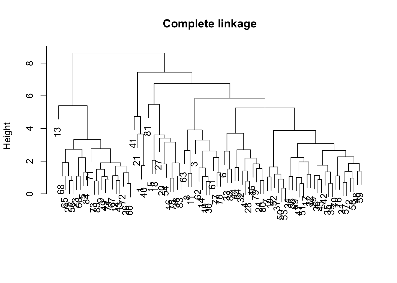
Note that the order in which the different branches are shown in the graph is arbitrary. What is relevant is what happens at each height of the tree, i.e., which observations are grouped together and then grouped as a cluster with other observations.
Determining clusters
Actual clusters are determined by cutting the tree at a given height. This is accomplished using the cutree command. The arguments are the hclust object (hc1 in our example) and the number of clusters. First, we use 4.
hc1_4 <- cutree(hc1,4)
hc1_4
## [1] 1 2 2 2 3 2 2 2 3 2 2 3 3 2 4 4 2 4 2 4 1 2 3 2 3 3 4 2 2 2 2 2 2 2 2
## [36] 2 2 4 2 1 1 2 3 2 2 2 2 2 3 2 2 2 2 4 3 2 2 2 2 3 2 2 2 2 3 3 3 3 2 2
## [71] 3 3 3 3 4 2 2 2 2 2 4 2 4 3 3The result is a vector that shows for each observation which cluster it belongs to. Note that the labels are irrelevant, only the grouping is. So, we could easily change 1 to 2 and 2 to 1 without affecting the result.
A useful summary is to use the table command which shows how many observations are included in each cluster.
table(hc1_4)## hc1_4
## 1 2 3 4
## 4 50 21 10Similarly, we can use cutree to find out how observations group themselves into 6 clusters.
hc1_6 <- cutree(hc1,6)
hc1_6
## [1] 1 2 3 2 4 2 2 3 4 3 3 4 4 3 5 5 2 5 2 5 1 2 4 2 4 4 5 2 2 3 2 2 2 2 2
## [36] 2 2 5 2 1 1 2 4 2 2 2 2 2 4 2 2 2 2 5 4 2 2 2 2 4 3 3 3 2 4 4 4 4 2 2
## [71] 4 4 4 4 5 2 3 3 2 2 6 2 5 4 4table(hc1_6)## hc1_6
## 1 2 3 4 5 6
## 4 39 11 21 9 1We now have a singleton in cluster 6.
Single linkage
We now repeat the procedure using the single linkage option. Everything (except the results) is the same as before, so we simply provide the output.
hc2 <- hclust(vdist,method="single")plot(hc2,main="Single linkage",xlab="",sub="")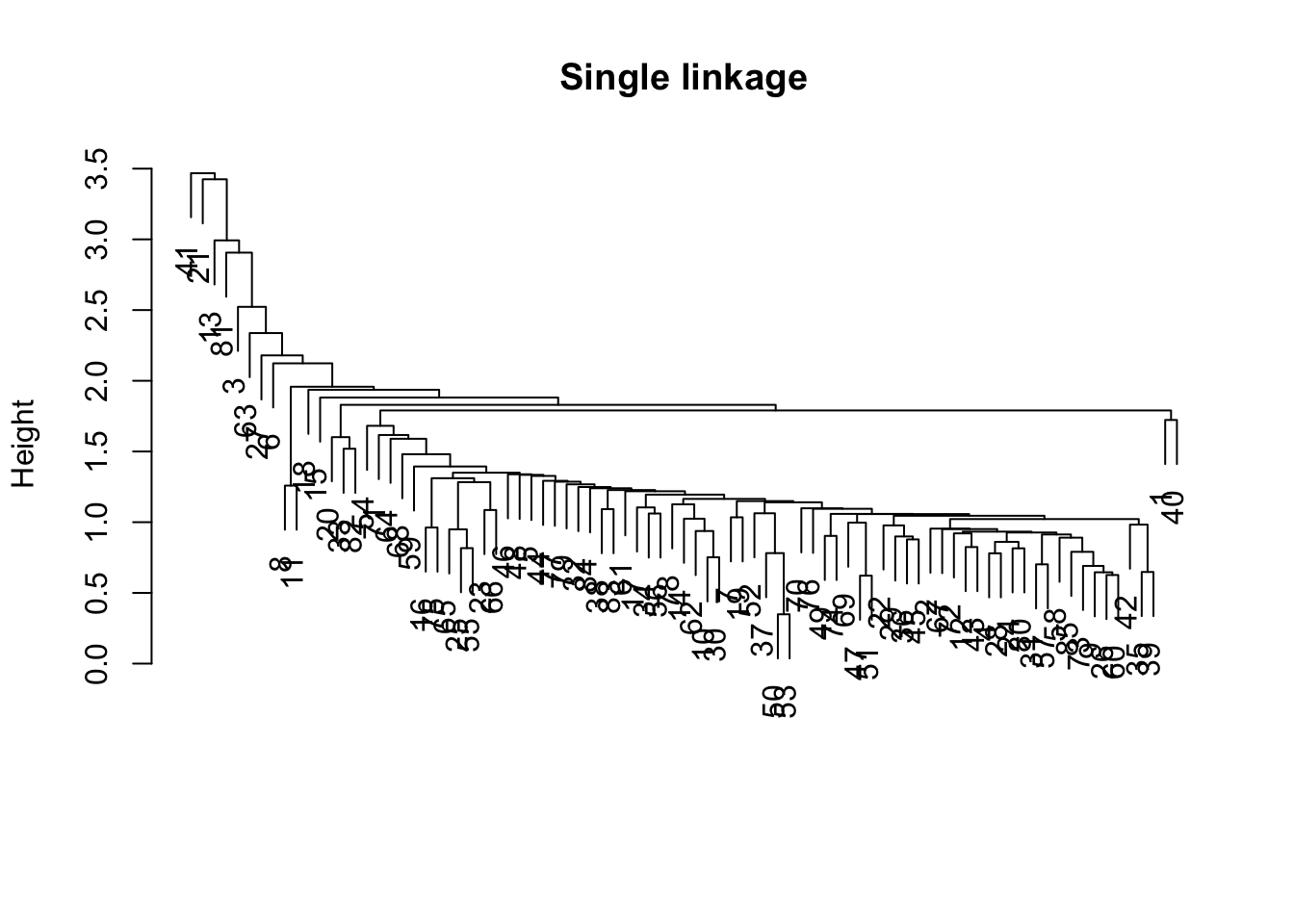
The dendrogram shows a characteristic form for single linkage, with one large cluster containing many (most) observations, and a few minor clusters and singletons.
We can check this with the cutree command.
hc2_4 <- cutree(hc2,4)
hc2_4
## [1] 1 1 1 1 1 1 1 1 1 1 1 1 2 1 1 1 1 1 1 1 3 1 1 1 1 1 1 1 1 1 1 1 1 1 1
## [36] 1 1 1 1 1 4 1 1 1 1 1 1 1 1 1 1 1 1 1 1 1 1 1 1 1 1 1 1 1 1 1 1 1 1 1
## [71] 1 1 1 1 1 1 1 1 1 1 1 1 1 1 1And using table to obtain the cluster frequencies.
table(hc2_4)## hc2_4
## 1 2 3 4
## 82 1 1 1The clusters are characterized by three singletons.
hc2_6 <- cutree(hc2,6)
hc2_6
## [1] 1 1 2 1 1 1 1 1 1 1 1 1 3 1 1 1 1 1 1 1 4 1 1 1 1 1 1 1 1 1 1 1 1 1 1
## [36] 1 1 1 1 1 5 1 1 1 1 1 1 1 1 1 1 1 1 1 1 1 1 1 1 1 1 1 1 1 1 1 1 1 1 1
## [71] 1 1 1 1 1 1 1 1 1 1 6 1 1 1 1table(hc2_6)## hc2_6
## 1 2 3 4 5 6
## 80 1 1 1 1 1Again, the frequency distribution is dominated by singletons.
We can now proceed in the same way as illustrated in the previous notebook to turn the cluster categories into variables that are part of a data frame, add the ID for the departments, and write to a csv file for later merging with the Guerry layer in GeoDa (see below for an example using the kmeans results).
The same mapping can also be achieved in R, by means of the maptools and other packages and reading in the shape file rather than the dbf file, but a treatment of this is beyond our current scope.
K-means clustering
K-means is an example of so-called partitioning clustering methods. These start with an initial assignment of observations to a given number of groupings (k). Since this initial assignment is random, it may be difficult to replicate the results of a particular application exactly. As we have seen before, the way we handle this is by setting a random seed. As a result, the series of random numbers that follows will always be the same.
In addition, to avoid getting trapped in a local optimum, it is good practice to start with several initial random assignments and then to pick the best of them to proceed.
In the kmeans function, this is accomplished by setting the nstart argument. The main argument to kmeans is a matrix with observations on the variables we want to consider, in our example, we use the standardized values in vds. This is followed by the number of desired clusters, k. Each time, we preceed the kmeans command by a set.seed function to ensure replicability.
k = 4
In our first example, we use k=4 and 20 initial random assignments (nstart=20).
set.seed(123456789)
km1_4 <- kmeans(vds,4,nstart=20)
The resulting object is of class kmeans. Again, we can investigate its type and contents by means of the class and str commands.
class(km1_4)## [1] "kmeans"str(km1_4)## List of 9
## $ cluster : int [1:85] 1 2 1 3 2 3 2 1 2 3 ...
## $ centers : num [1:4, 1:6] -0.0186 0.2256 -0.4565 0.2456 1.5041 ...
## ..- attr(*, "dimnames")=List of 2
## .. ..$ : chr [1:4] "1" "2" "3" "4"
## .. ..$ : chr [1:6] "Crm_prs" "Crm_prp" "Litercy" "Donatns" ...
## $ totss : num 504
## $ withinss : num [1:4] 62.5 87.4 57.7 77.8
## $ tot.withinss: num 285
## $ betweenss : num 219
## $ size : int [1:4] 10 34 25 16
## $ iter : int 3
## $ ifault : int 0
## - attr(*, "class")= chr "kmeans"The cluster component lists the membership of each observation in one of the clusters. As before, the labeling is arbitrary. centers show the coordinates of the cluster centers (depending on the method), i.e. the value for each of the six variables we considered. Next follow a series of sum of squares measures, i.e., the total totss, the within sum of squares for each cluster (withinss), the total within sum of squares (tot.withinss), and the between sum of squares (betweenss). Finally, the size of each cluster is contained in the size component.
In this particular implementation, the summary command is not that meaningful, but a simple listing of the object provides the most important information.
km1_4## K-means clustering with 4 clusters of sizes 10, 34, 25, 16
##
## Cluster means:
## Crm_prs Crm_prp Litercy Donatns Infants Suicids
## 1 -0.01862401 1.50414480 -0.6677156 -0.2295418 0.34602027 2.06436732
## 2 0.22555526 -0.55018807 0.9450588 -0.2202584 -0.58660877 -0.56073786
## 3 -0.45646127 0.19707925 -0.4853169 -0.5625622 0.08631219 -0.03040797
## 4 0.24555582 -0.07887718 -0.8326200 1.4905163 0.89541817 -0.05114916
##
## Clustering vector:
## [1] 1 2 1 3 2 3 2 1 2 3 1 2 4 1 4 4 4 4 2 4 1 3 2 3 2 2 4 3 3 3 2 3 4 4 3
## [36] 3 2 4 3 1 1 3 2 3 3 3 3 2 2 2 3 2 2 4 2 4 2 2 2 2 1 3 1 3 2 2 2 2 3 2
## [71] 2 2 2 2 4 2 3 3 3 3 4 4 4 2 2
##
## Within cluster sum of squares by cluster:
## [1] 62.54998 87.39083 57.68289 77.75905
## (between_SS / total_SS = 43.4 %)
##
## Available components:
##
## [1] "cluster" "centers" "totss" "withinss"
## [5] "tot.withinss" "betweenss" "size" "iter"
## [9] "ifault"For future manipulation, we assign the resulting classification to a vector.
k4 <- km1_4$cluster
k4
## [1] 1 2 1 3 2 3 2 1 2 3 1 2 4 1 4 4 4 4 2 4 1 3 2 3 2 2 4 3 3 3 2 3 4 4 3
## [36] 3 2 4 3 1 1 3 2 3 3 3 3 2 2 2 3 2 2 4 2 4 2 2 2 2 1 3 1 3 2 2 2 2 3 2
## [71] 2 2 2 2 4 2 3 3 3 3 4 4 4 2 2We can assess the sensitivity of the result (and the extent to which it may be a local optimum) by starting with a different seed and trying more initial assignments, such as nstart=50.
set.seed(987654321)
km1_4a <- kmeans(vds,4,nstart=50)km1_4a## K-means clustering with 4 clusters of sizes 10, 34, 25, 16
##
## Cluster means:
## Crm_prs Crm_prp Litercy Donatns Infants Suicids
## 1 -0.01862401 1.50414480 -0.6677156 -0.2295418 0.34602027 2.06436732
## 2 0.22555526 -0.55018807 0.9450588 -0.2202584 -0.58660877 -0.56073786
## 3 -0.45646127 0.19707925 -0.4853169 -0.5625622 0.08631219 -0.03040797
## 4 0.24555582 -0.07887718 -0.8326200 1.4905163 0.89541817 -0.05114916
##
## Clustering vector:
##  [1] 1 2 1 3 2 3 2 1 2 3 1 2 4 1 4 4 4 4 2 4 1 3 2 3 2 2 4 3 3 3 2 3 4 4 3
## [36] 3 2 4 3 1 1 3 2 3 3 3 3 2 2 2 3 2 2 4 2 4 2 2 2 2 1 3 1 3 2 2 2 2 3 2
## [71] 2 2 2 2 4 2 3 3 3 3 4 4 4 2 2
##
## Within cluster sum of squares by cluster:
## [1] 62.54998 87.39083 57.68289 77.75905
## (between_SS / total_SS = 43.4 %)
##
## Available components:
##
## [1] "cluster" "centers" "totss" "withinss"
## [5] "tot.withinss" "betweenss" "size" "iter"
## [9] "ifault"We see that the results are the same.
k = 6
In parallel to what we did for hierarchical clustering, we now set the number of clusters to 6. The operations are identical to what we just covered, so we only list the output.
set.seed(123456789)
km1_6 <- kmeans(vds,6,nstart=20)
km1_6
## K-means clustering with 6 clusters of sizes 18, 12, 18, 22, 5, 10
##
## Cluster means:
## Crm_prs Crm_prp Litercy Donatns Infants Suicids
## 1 1.08996145 0.04903608 0.7566768 -0.2830040 -0.4135130 -0.3877974
## 2 0.25047928 0.04996547 -0.8111108 1.7451174 0.2653963 -0.2374746
## 3 -0.52568581 -1.02513101 0.9542435 -0.1938888 -0.6870929 -0.7022251
## 4 -0.56649536 0.13677587 -0.4591407 -0.5564466 -0.0268111 -0.0324456
## 5 -0.10271494 -0.21607881 -0.8569972 0.4359810 2.7511582 0.5080462
## 6 -0.01862401 1.50414480 -0.6677156 -0.2295418 0.3460203 2.0643673
##
## Clustering vector:
##  [1] 6 1 6 4 3 5 1 6 3 4 6 3 2 6 2 2 2 2 1 5 6 4 3 4 3 3 2 4 4 4 1 4 5 2 4
## [36] 4 1 2 4 6 6 4 3 4 4 4 1 1 3 1 4 1 1 2 3 2 1 1 1 3 6 4 6 4 3 3 3 1 1 1
## [71] 3 3 3 3 2 1 4 4 4 4 5 5 2 1 3
##
## Within cluster sum of squares by cluster:
## [1] 32.06555 41.60399 30.35707 42.23770 16.71851 62.54998
## (between_SS / total_SS = 55.3 %)
##
## Available components:
##
## [1] "cluster" "centers" "totss" "withinss"
## [5] "tot.withinss" "betweenss" "size" "iter"
## [9] "ifault"k6 <- km1_6$cluster
k6## [1] 6 1 6 4 3 5 1 6 3 4 6 3 2 6 2 2 2 2 1 5 6 4 3 4 3 3 2 4 4 4 1 4 5 2 4
## [36] 4 1 2 4 6 6 4 3 4 4 4 1 1 3 1 4 1 1 2 3 2 1 1 1 3 6 4 6 4 3 3 3 1 1 1
## [71] 3 3 3 3 2 1 4 4 4 4 5 5 2 1 3Cluster output for merging with GeoDa
As an illustration, we follow the same procedure as before to create a data frame with an ID variable for output to a csv file. That file can then be merged into a geographical layer in GeoDa.
kmdat <- as.data.frame(cbind(k4,k6))
kmdat$IDK <- dat$dept
write.csv(kmdat,"kmeansclus.csv",row.names=FALSE)
University of Chicago, Center for Spatial Data Science – anselin@uchicago.edu↩