Introduction
We will consider principal components analysis (PCA) and multidimensional scaling (MDS) as examples of multivariate dimension reduction. Both techniques are included in the base R installation, respectively as prcomp and cmdscale. We will also use the (best practice) graphics package ggplot2 for our plots.
We will use the Guerry_85 file that contains observations on socio-economic characteristics for the 85 French departments in 1830.
Note: this is written with R beginners in mind, more seasoned R users can probably skip most of the comments on data structures and other R particulars. Also, as always in R, there are typically several ways to achieve a specific objective, so what is shown here is just one way that works, but there often are others (that may even work faster, or scale better).
Items covered:
scaling a multivariate data set (i.e., standardizing to mean zero and variance one) using scale
computing principal components using prcomp
extracting loadings, scores and proportion explained variance
creating a scree plot to assess the proportion variance explained and to select the number of meaningful components
using ggplot2 to create a scatter plot with meaningful labels
creating a biplot to interpret the relative contribution of two PC
computing multivariate distance using dist
carrying out multidimensional scaling using cmdscale
plotting the results of multi-dimensional scaling using ggplot2
Packages used:
foreign
ggplot2
Preliminaries
As is customary by now, we start by installing the required packages, read in the data, and provide a summary of the data. The input file is Guerry_85.dbf and we use read.dbf to turn it into an R data frame (your contents of the Guerry file may be slightly different).
library(foreign)
library(ggplot2)
dat <- read.dbf("Guerry_85.dbf")
summary(dat)## CODE_DE COUNT AVE_ID_ dept Region
## 01 : 1 Min. :1.000 Min. : 49 Min. : 1.00 C:17
## 02 : 1 1st Qu.:1.000 1st Qu.: 8612 1st Qu.:24.00 E:17
## 03 : 1 Median :1.000 Median :16732 Median :45.00 N:17
## 04 : 1 Mean :1.059 Mean :17701 Mean :45.08 S:17
## 05 : 1 3rd Qu.:1.000 3rd Qu.:26842 3rd Qu.:66.00 W:17
## 07 : 1 Max. :4.000 Max. :36521 Max. :89.00
## (Other):79
## Dprtmnt Crm_prs Crm_prp Litercy
## Ain : 1 Min. : 5883 Min. : 1368 Min. :12.00
## Aisne : 1 1st Qu.:14790 1st Qu.: 5990 1st Qu.:25.00
## Allier : 1 Median :18785 Median : 7624 Median :38.00
## Ardeche : 1 Mean :19961 Mean : 7881 Mean :39.14
## Ardennes: 1 3rd Qu.:26221 3rd Qu.: 9190 3rd Qu.:52.00
## Ariege : 1 Max. :37014 Max. :20235 Max. :74.00
## (Other) :79
## Donatns Infants Suicids MainCty
## Min. : 1246 Min. : 2660 Min. : 3460 Min. :1
## 1st Qu.: 3446 1st Qu.:14281 1st Qu.: 15400 1st Qu.:2
## Median : 4964 Median :17044 Median : 26198 Median :2
## Mean : 6723 Mean :18983 Mean : 36517 Mean :2
## 3rd Qu.: 9242 3rd Qu.:21981 3rd Qu.: 45180 3rd Qu.:2
## Max. :27830 Max. :62486 Max. :163241 Max. :3
##
## Wealth Commerc Clergy Crm_prn
## Min. : 1.00 Min. : 1.00 Min. : 2.00 Min. : 1.00
## 1st Qu.:22.00 1st Qu.:21.00 1st Qu.:23.00 1st Qu.:22.00
## Median :44.00 Median :42.00 Median :44.00 Median :43.00
## Mean :43.58 Mean :42.33 Mean :43.93 Mean :43.06
## 3rd Qu.:65.00 3rd Qu.:63.00 3rd Qu.:65.00 3rd Qu.:64.00
## Max. :86.00 Max. :86.00 Max. :86.00 Max. :86.00
##
## Infntcd Dntn_cl Lottery Desertn
## Min. : 1 Min. : 1.00 Min. : 1.00 Min. : 1.00
## 1st Qu.:23 1st Qu.:22.00 1st Qu.:22.00 1st Qu.:23.00
## Median :44 Median :43.00 Median :43.00 Median :44.00
## Mean :44 Mean :43.02 Mean :43.04 Mean :43.91
## 3rd Qu.:65 3rd Qu.:64.00 3rd Qu.:64.00 3rd Qu.:65.00
## Max. :86 Max. :86.00 Max. :86.00 Max. :86.00
##
## Instrct Prsttts Distanc Area
## Min. : 1.00 Min. : 0.0 Min. : 0.0 Min. : 762
## 1st Qu.:23.00 1st Qu.: 6.0 1st Qu.:119.7 1st Qu.: 5361
## Median :42.00 Median : 34.0 Median :199.2 Median : 6040
## Mean :43.34 Mean : 143.5 Mean :204.1 Mean : 6117
## 3rd Qu.:65.00 3rd Qu.: 117.0 3rd Qu.:283.8 3rd Qu.: 6815
## Max. :86.00 Max. :4744.0 Max. :403.4 Max. :10000
##
## Pop1831 CL_CRMP CL_CRPROP CL_LIT
## Min. :129.1 Min. :0.0000 Min. :0.0000 Min. :0.0000
## 1st Qu.:283.8 1st Qu.:0.0000 1st Qu.:0.0000 1st Qu.:0.0000
## Median :346.3 Median :0.0000 Median :0.0000 Median :0.0000
## Mean :380.8 Mean :0.5412 Mean :0.3412 Mean :0.6706
## 3rd Qu.:445.2 3rd Qu.:1.0000 3rd Qu.:0.0000 3rd Qu.:1.0000
## Max. :989.9 Max. :3.0000 Max. :3.0000 Max. :2.0000
##
## CL_DON CL_Inf CL_SUIC BX_CRMP
## Min. :0.0000 Min. :0.0000 Min. :0.0000 Min. :2.000
## 1st Qu.:0.0000 1st Qu.:0.0000 1st Qu.:0.0000 1st Qu.:3.000
## Median :0.0000 Median :0.0000 Median :0.0000 Median :4.000
## Mean :0.6588 Mean :0.3412 Mean :0.6235 Mean :3.506
## 3rd Qu.:1.0000 3rd Qu.:0.0000 3rd Qu.:1.0000 3rd Qu.:4.000
## Max. :4.0000 Max. :4.0000 Max. :3.0000 Max. :5.000
##
## BX_CRMPROP BX_LIT BX_DON BX_INF
## Min. :2.000 Min. :2.000 Min. :2.000 Min. :1.000
## 1st Qu.:3.000 1st Qu.:3.000 1st Qu.:3.000 1st Qu.:3.000
## Median :4.000 Median :4.000 Median :4.000 Median :4.000
## Mean :3.541 Mean :3.518 Mean :3.529 Mean :3.553
## 3rd Qu.:4.000 3rd Qu.:4.000 3rd Qu.:4.000 3rd Qu.:4.000
## Max. :6.000 Max. :5.000 Max. :6.000 Max. :6.000
##
## BX_SUIC AREA_ID PC1 PC2
## Min. :2.000 Min. : 1.00 Min. :-4.76964 Min. :-2.406826
## 1st Qu.:3.000 1st Qu.:24.00 1st Qu.:-0.99525 1st Qu.:-0.771465
## Median :4.000 Median :45.00 Median : 0.05716 Median : 0.000518
## Mean :3.565 Mean :45.08 Mean : 0.00000 Mean : 0.000000
## 3rd Qu.:4.000 3rd Qu.:66.00 3rd Qu.: 1.09196 3rd Qu.: 0.644247
## Max. :6.000 Max. :89.00 Max. : 3.49999 Max. : 3.725174
##
## PC3 PC4 PC5
## Min. :-3.138126 Min. :-2.73920 Min. :-1.312376
## 1st Qu.:-0.700550 1st Qu.:-0.40852 1st Qu.:-0.551329
## Median : 0.005259 Median : 0.04634 Median : 0.005071
## Mean : 0.000000 Mean : 0.00000 Mean : 0.000000
## 3rd Qu.: 0.802456 3rd Qu.: 0.50856 3rd Qu.: 0.383585
## Max. : 2.299306 Max. : 2.43883 Max. : 2.025063
##
## PC6
## Min. :-1.67472
## 1st Qu.:-0.31903
## Median :-0.01997
## Mean : 0.00000
## 3rd Qu.: 0.33713
## Max. : 1.42404
## Extracting the variables
We will extract a subset of the variables included in the data frame for use in the PCA. First, we define a list with all the variable names, and then we use the standard column subsetting of the initial data frame (note the empty space before the comma to specify that we select all observations or rows). We also summarize the new data frame.
varnames <- c("Crm_prs","Crm_prp","Litercy","Donatns","Infants","Suicids")
vd1 <- dat[,varnames]
summary(vd1)
## Crm_prs Crm_prp Litercy Donatns
## Min. : 5883 Min. : 1368 Min. :12.00 Min. : 1246
## 1st Qu.:14790 1st Qu.: 5990 1st Qu.:25.00 1st Qu.: 3446
## Median :18785 Median : 7624 Median :38.00 Median : 4964
## Mean :19961 Mean : 7881 Mean :39.14 Mean : 6723
## 3rd Qu.:26221 3rd Qu.: 9190 3rd Qu.:52.00 3rd Qu.: 9242
## Max. :37014 Max. :20235 Max. :74.00 Max. :27830
## Infants Suicids
## Min. : 2660 Min. : 3460
## 1st Qu.:14281 1st Qu.: 15400
## Median :17044 Median : 26198
## Mean :18983 Mean : 36517
## 3rd Qu.:21981 3rd Qu.: 45180
## Max. :62486 Max. :163241Standardizing the variables
We standardize the variables by means of the scale command. We again also provide a summary. Obviously, the mean is zero for all variables. We check the variance for one selected variable (Crm_prs) and it is indeed one.
Note that the resulting object is a matrix and not a data.frame (the $ notation does not work to extract the Crm_prs column). We specify the column explicitly by giving its name (in quotes), preceded by a comma with empty space before the comma (meaning all the rows are selected).
vds <- scale(vd1)
summary(vds)
## Crm_prs Crm_prp Litercy Donatns
## Min. :-1.9287 Min. :-2.13649 Min. :-1.55677 Min. :-1.1263
## 1st Qu.:-0.7084 1st Qu.:-0.62039 1st Qu.:-0.81111 1st Qu.:-0.6739
## Median :-0.1611 Median :-0.08441 Median :-0.06546 Median :-0.3618
## Mean : 0.0000 Mean : 0.00000 Mean : 0.00000 Mean : 0.0000
## 3rd Qu.: 0.8576 3rd Qu.: 0.42926 3rd Qu.: 0.73756 3rd Qu.: 0.5179
## Max. : 2.3363 Max. : 4.05222 Max. : 1.99944 Max. : 4.3400
## Infants Suicids
## Min. :-1.8443 Min. :-1.0495
## 1st Qu.:-0.5313 1st Qu.:-0.6704
## Median :-0.2191 Median :-0.3276
## Mean : 0.0000 Mean : 0.0000
## 3rd Qu.: 0.3387 3rd Qu.: 0.2750
## Max. : 4.9153 Max. : 4.0232var(vds[,"Crm_prs"])## [1] 1Principal Component Analysis
The computations for PCA are carried out by means of the prcomp function. Since we already scaled our variables, we do not need to specify this as an argument and the only item passed to the function is the name of the matrix containing the scaled variables, vds in our example (see the help file for other options).
prc <- prcomp(vds)The result of this computation is an object of the special class prcomp. It contains lots of information, which we can check with the usual str command.
class(prc)## [1] "prcomp"str(prc)## List of 5
## $ sdev : num [1:6] 1.463 1.096 1.05 0.817 0.741 ...
## $ rotation: num [1:6, 1:6] -0.0659 -0.5123 0.5118 -0.1062 -0.4513 ...
## ..- attr(*, "dimnames")=List of 2
## .. ..$ : chr [1:6] "Crm_prs" "Crm_prp" "Litercy" "Donatns" ...
## .. ..$ : chr [1:6] "PC1" "PC2" "PC3" "PC4" ...
## $ center : Named num [1:6] 1.18e-16 9.16e-17 2.39e-17 7.52e-17 1.91e-16 ...
## ..- attr(*, "names")= chr [1:6] "Crm_prs" "Crm_prp" "Litercy" "Donatns" ...
## $ scale : Named num [1:6] 7299.2 3048.6 17.4 4863.2 8850.6 ...
## ..- attr(*, "names")= chr [1:6] "Crm_prs" "Crm_prp" "Litercy" "Donatns" ...
## $ x : num [1:85, 1:6] -2.151 1.246 -2.077 0.604 0.963 ...
## ..- attr(*, "dimnames")=List of 2
## .. ..$ : NULL
## .. ..$ : chr [1:6] "PC1" "PC2" "PC3" "PC4" ...
## - attr(*, "class")= chr "prcomp"A summary of the principal component object yields the standard deviation associated with each component (the variance corresponds to the eigenvalue), and the corresponding proportion and cumulative proportion of the explained variance. The standard deviations are also contained in the sdev attribute.
summary(prc)## Importance of components%s:
## PC1 PC2 PC3 PC4 PC5 PC6
## Standard deviation 1.4630 1.0958 1.0498 0.8167 0.74073 0.58397
## Proportion of Variance 0.3568 0.2001 0.1837 0.1112 0.09145 0.05684
## Cumulative Proportion 0.3568 0.5569 0.7406 0.8517 0.94316 1.00000The standard deviation can also be extracted separately as dev.
prc$sdev## [1] 1.4630347 1.0958193 1.0497842 0.8166799 0.7407260 0.5839706The results are not that great. Three components (out of six!) are needed to explain 75% of the variance, and even five do not explain 95%. This is due largely to the low correlation among the variables (cor).
cor(vds)## Crm_prs Crm_prp Litercy Donatns Infants
## Crm_prs 1.00000000 0.25520756 -0.0206305 0.13362485 -0.02747066
## Crm_prp 0.25520756 1.00000000 -0.3628642 -0.08206739 0.27816055
## Litercy -0.02063050 -0.36286419 1.0000000 -0.19576462 -0.41233536
## Donatns 0.13362485 -0.08206739 -0.1957646 1.00000000 0.15912057
## Infants -0.02747066 0.27816055 -0.4123354 0.15912057 1.00000000
## Suicids -0.13427098 0.52334916 -0.3742741 -0.03485190 0.28863250
## Suicids
## Crm_prs -0.1342710
## Crm_prp 0.5233492
## Litercy -0.3742741
## Donatns -0.0348519
## Infants 0.2886325
## Suicids 1.0000000Scree plot
The scree plot shows the proportion variance explained as a decreasing function of the principal components (each component explains a little less than the previous component). This is used to “eyeball” a reasonable number of components to use in further analysis. Note that there is no point to using all the principal components because then there would be no dimension reduction. The whole objective is to capture most of the variance in the data by means of a small number of components.
To select this number, one looks for an elbow or kink in the scree plot, i.e., a meaningful change in the slope such that the additional variance explained is small relative to the previous PC.
The prcomp function does not include an explicit function to create a scree plot, but it is relatively straightfoward to write a small function to accomplish this goal. The function scree_plot below does just that.
scree_plot <- function(princ,cumulative=FALSE)
    {
    pv <- princ$sdev^2
    pve <- pv / sum(pv)
    mtitle="Scree Plot"
    if (cumulative){
        pve <- cumsum(pve)
        mtitle="Cumulative Variance Proportion"
    }
    plot(pve,type="b",main=mtitle,xlab="Principal Components",
         ylab="Proportion Variance Explained")
}
The function takes as argument the principal component object. The default is to create a scree plot. However, setting the option cumulative=TRUE creates the complement, i.e., a curve showing the cumulative variance explained. Note how that is computed using the cumsum command in the function. The plot is a simple line plot (type = “b”) with titles appropriate for each plot (this illustrates the use of if).
In our example, the scree plot is created using scree_plot(prc), as shown below.
scree_plot(prc)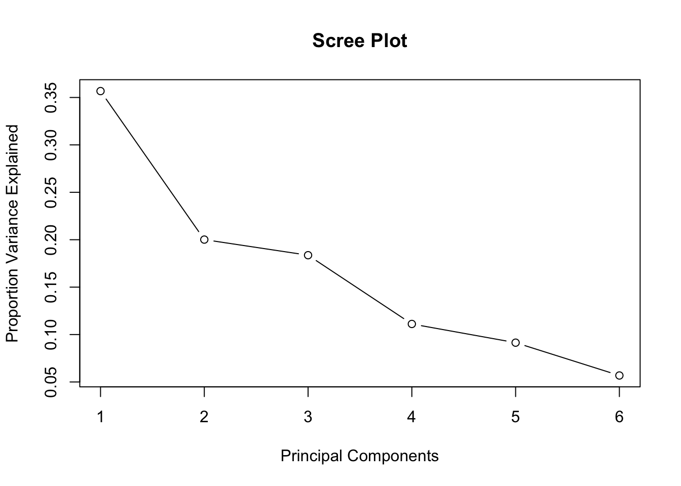
Unlike most textbook examples, this plot does not have a clear kink. In part, this is due to the low correlations between the variables, which does not lend itself to identifying common dimensions that explain a lot of the underlying variance.
The graph with the cumulative proportion of the explained variable is obtained by setting cumulative=TRUE, as shown below.
scree_plot(prc,cumulative=TRUE)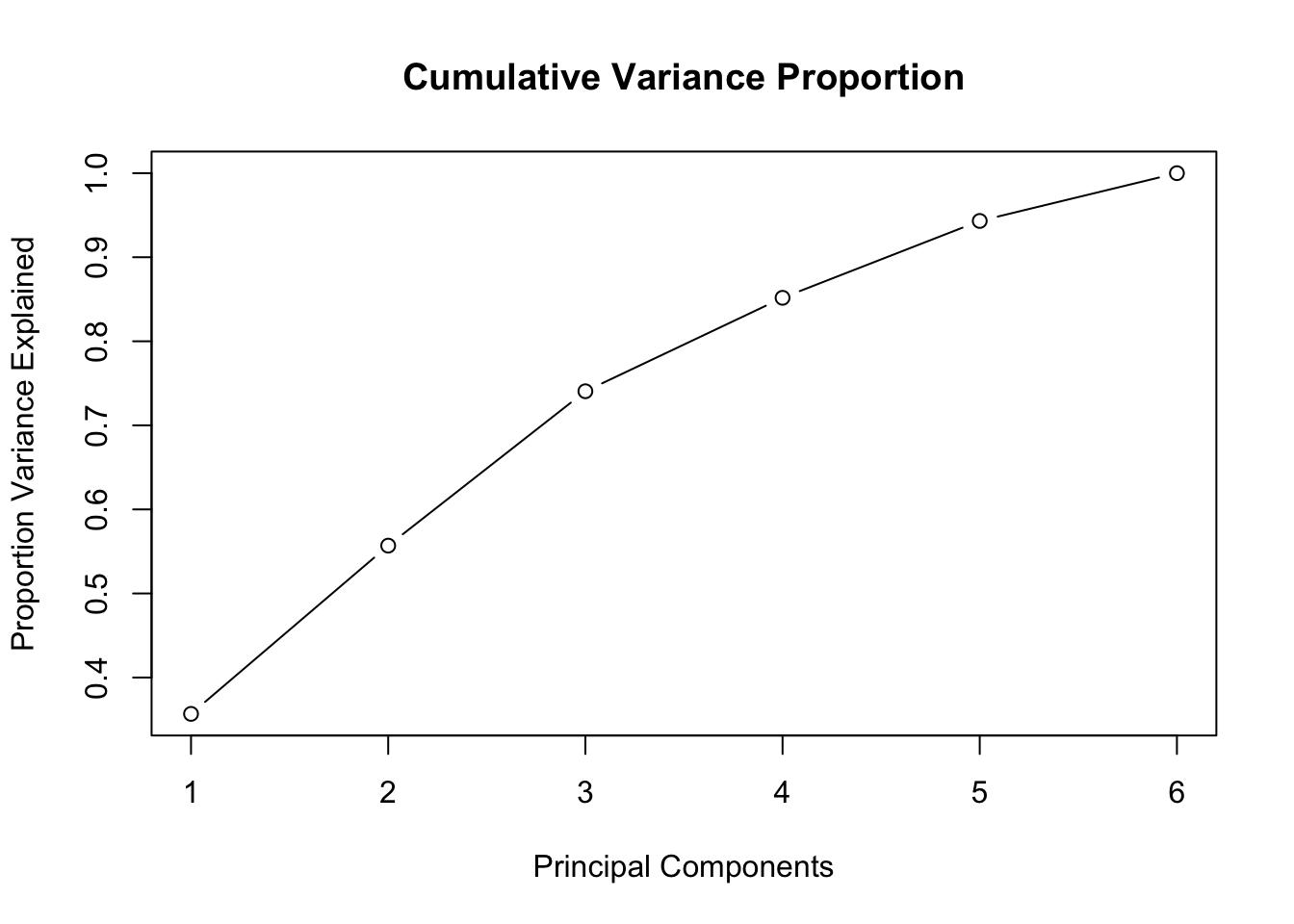
Here again, there is no clear kink. This is a graphical description of the variance proportions we saw above.
Loadings
The loadings (i.e., the coefficients that apply to each of the original variables to obtain the principal component score for an observation) are contained in the rotation attribute of the PC object. We extract in the usual fashion. The loadings are the row elements for each of the columns of the matrix that correspond to a principal component.
pcld <- prc$rotation
pcld
## PC1 PC2 PC3 PC4 PC5
## Crm_prs -0.06586882 0.59059665 -0.67318936 0.139728619 -0.01017718
## Crm_prp -0.51232573 -0.08836869 -0.47654080 -0.098606014 0.13805617
## Litercy 0.51175292 -0.12936154 -0.20902824 0.007966705 0.82126885
## Donatns -0.10619494 0.69899915 0.41339634 -0.472983512 0.27420690
## Infants -0.45133749 0.10331305 0.32380799 0.730309102 0.37758929
## Suicids -0.50627038 -0.35690163 -0.01685224 -0.462195317 0.29764289
## PC6
## Crm_prs -0.41718740
## Crm_prp 0.68836003
## Litercy 0.05599763
## Donatns 0.17413633
## Infants -0.06960037
## Suicids -0.56018901The interpretation of the loadings can be tricky, but sometimes there is a clear interpretation when only a subset of the variables shows high values for the coefficients, or when the signs for a given variable are very different between the components. We return to this below when we consider the biplot.
More informative than the loadings is the matrix of squared correlations between the original variables and the principal components. We return to this below.
Principal component scores
The score for a principal component for each observation is obtained by multiplying the original values for the variables that went into the components by the matching loading (remember that all the variables were standardized, so it is the standardized version that gets multiplied by the loadings). A small number of these principal component scores can then be used instead of the full set of variables to represent a sizeable fraction of the variance in the data.
The component scores can be used as regular variables, in that they can be plotted, mapped, etc. However, keep in mind that they are orthogonal by construction, so the slope in a bivariate scatter plot of two components will always be zero (i.e., the linear fit will be a horizontal line).
The scores are contained in the x attribute of the principal component object.
pcscores <- prc$x
summary(pcscores)
## PC1 PC2 PC3
## Min. :-4.76964 Min. :-2.406826 Min. :-3.138126
## 1st Qu.:-0.99525 1st Qu.:-0.771465 1st Qu.:-0.700550
## Median : 0.05716 Median : 0.000518 Median : 0.005259
## Mean : 0.00000 Mean : 0.000000 Mean : 0.000000
## 3rd Qu.: 1.09196 3rd Qu.: 0.644247 3rd Qu.: 0.802456
## Max. : 3.49999 Max. : 3.725174 Max. : 2.299306
## PC4 PC5 PC6
## Min. :-2.73920 Min. :-1.312376 Min. :-1.67472
## 1st Qu.:-0.40852 1st Qu.:-0.551329 1st Qu.:-0.31903
## Median : 0.04634 Median : 0.005071 Median :-0.01997
## Mean : 0.00000 Mean : 0.000000 Mean : 0.00000
## 3rd Qu.: 0.50856 3rd Qu.: 0.383585 3rd Qu.: 0.33713
## Max. : 2.43883 Max. : 2.025063 Max. : 1.42404They are contained in a class matrix.
class(pcscores)## [1] "matrix"And, of course, are uncorrelated.
cor(pcscores)## PC1 PC2 PC3 PC4 PC5
## PC1 1.000000e+00 1.545200e-16 -1.674485e-17 -1.464190e-16 -4.136780e-16
## PC2 1.545200e-16 1.000000e+00 -5.064932e-16 8.149796e-17 -1.758957e-16
## PC3 -1.674485e-17 -5.064932e-16 1.000000e+00 2.379312e-16 -1.273930e-16
## PC4 -1.464190e-16 8.149796e-17 2.379312e-16 1.000000e+00 2.058558e-16
## PC5 -4.136780e-16 -1.758957e-16 -1.273930e-16 2.058558e-16 1.000000e+00
## PC6 -1.147708e-15 -3.651595e-16 -4.990062e-16 -7.126695e-16 3.643055e-16
## PC6
## PC1 -1.147708e-15
## PC2 -3.651595e-16
## PC3 -4.990062e-16
## PC4 -7.126695e-16
## PC5 3.643055e-16
## PC6 1.000000e+00A more informative way to interpret the connection between the original variables and the scores is the squared correlation matrix.
vv <- cor(vds,pcscores)
vv2 <- vv**2
vv2
## PC1 PC2 PC3 PC4 PC5
## Crm_prs 0.009286863 0.418851254 0.4994299246 1.302190e-02 5.682901e-05
## Crm_prp 0.561825664 0.009377232 0.2502650773 6.485009e-03 1.045747e-02
## Litercy 0.560570048 0.020095011 0.0481515209 4.233126e-05 3.700717e-01
## Donatns 0.024138865 0.586720363 0.1883359996 1.492093e-01 4.125456e-02
## Infants 0.436025658 0.012817054 0.1155513985 3.557273e-01 7.822662e-02
## Suicids 0.548623327 0.152958961 0.0003129792 1.424803e-01 4.860783e-02
## PC6
## Crm_prs 0.059353225
## Crm_prp 0.161589543
## Litercy 0.001069353
## Donatns 0.010340957
## Infants 0.001651981
## Suicids 0.107016596The elements along each row give the proportion of the variance of the variable in that row explained by the respective principal component. The values in each column for a principal component give the squared correlation between the original variable and that component, suggesting the relative importance of the former in interpreting the latter.
The sum across each of the rows (i.e., variables) equals 1.
rowSums(vv2)## Crm_prs Crm_prp Litercy Donatns Infants Suicids
## 1 1 1 1 1 1Converting the scores to a data frame
As we saw above, the scores are a matrix object, not a data frame. If we want to output these results (e.g., to join with a map in GeoDa), we need to turn them into a data frame.
In the few lines below, we first create a data frame from the matrix and then add the department ID (dept) as an additional variable. The resulting data frame can be written out to a csv file using write.csv and it can also be used by the plotting commands in ggplot (see further below).
pcs1 <- as.data.frame(pcscores)
pcs1$AREA_ID <- as.integer(dat$dept)
names(pcs1)
## [1] "PC1" "PC2" "PC3" "PC4" "PC5" "PC6" "AREA_ID"Plotting the PC scores
We can now construct a scatter plot for any pair of principal component scores. For example, below we use ggplot to easily add the labels corresponding to the departments to the plot. It turns out this is a bit tricky in the standard plot command, and it gives us an excuse to start exploring the functionality of ggplot.
The ggplot grammar follows Wilkinson’s grammar of graphics, which is an elegant way to abstract the construction of a wide array of statistical graphs. A characteristic of the ggplot approach is that a graph is created incrementally. In its bare bones essentials, there are two commands. First is the specification of the data and variables for the plot, entered as arguments to the ggplot command. In our case, the data set is the just created pcs1 and the two components PC1 and PC2 that correspond to the x and y coordinates in the plot. In ggplot, this is specified through the aes attribute (for aesthetics).
Beyond this first command, a graph is built up by adding (litterally, using the + sign) different geometric objects. In our case, we specify that the graph is a point graph (for x-y coordinates, this will give a scatter plot) by means of geom_point (all the different types are prefaced by geom). In addition, we add the labels as text using geom_text. We specify the AREA_ID as the label (as part of an aes attribute) and we use nudge-y to move the label above the point (the default is to have it listed on top of the point). For further specifics and options to make this look really fancy, check out the documentation of ggplot2 (or the excellent book on this package by its creator, Hadley Wickham).
ggplot(pcs1,aes(x=PC1,y=PC2)) +
geom_point() + geom_text(aes(label=AREA_ID),nudge_y=+0.3) 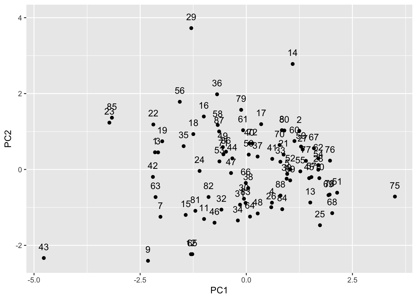
We can write the data frame to a csv file (using write.csv) and then merge this with a layer for the French departments in the Guerry layer in GeoDa. Using linking and brushing, we can examine the extent to which neighbors in multivariate space (points close together in the scatter plot) are also geographical neighbors. We will revisit this issue when we deal with clusters.
Biplot
An alternative way to visualize the results of a principal components analysis is by means of a so-called biplot. For any pair of components, this combines the scatter plot with a set of vectors showing the loadings for each variable. The vector is centered at zero. Its x dimension shows the importance of the loading for that variable for the principal component on the x-axis. The y dimension does the same for the component on the y-axis.
An easy case to interpret is when the loading is large for one component and small for the other, which will result in a very steep curve. Other easy cases are when the signs of the loadings are opposite. For example, a positive sign for PC1 and a negative sign for PC2 would give a vector pointing down and to the right. The information in the biplot confirms what we saw earlier in the matrix of squared correlations.
The biplot is invoked by the biplot command. The default is to plot the first two components, so that the only argument to the function is the principal component object. In our example, this is prc. We add the option scale=0 to make sure the arrows are scaled such that they reflect the loadings.
biplot(prc,scale=0)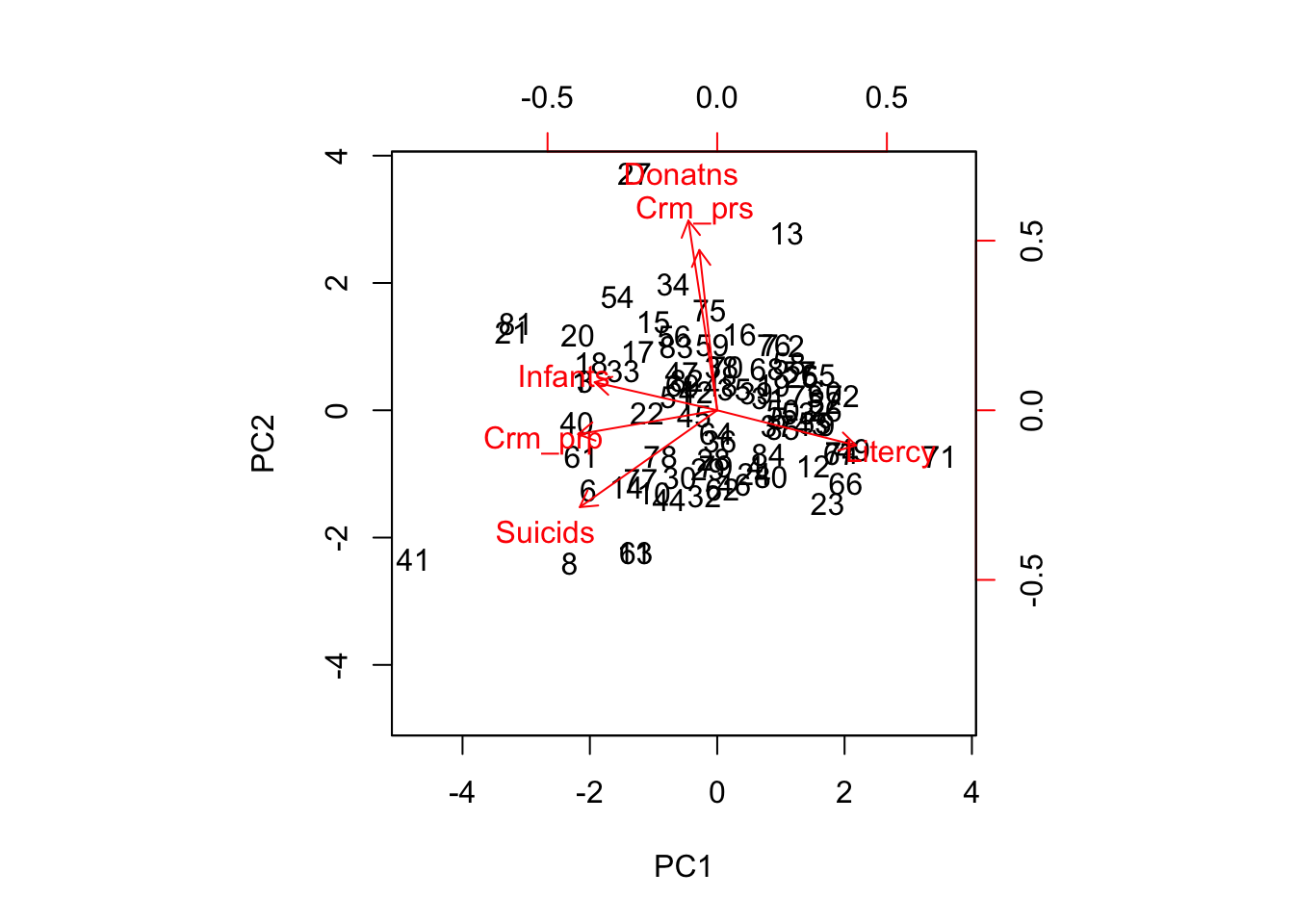
Multidimensional scaling
Multidimensional scaling consists of finding a lower dimensional representation of the data that respects the multidimensional distance between observation pairs as much as possible.
In R, this is computed using the cmdscale command. It takes as input a dissimilarity or distance matrix, computed using the dist command. As a default, this uses p-dimensional Euclidean distance, but several other options are available as well (see the documentation). In most circumstances, it is most appropriate the base the distance computation on standardized variables (use scale first).
The output of the MDS procedure is a matrix (not a data frame) with the coordinates in the lower-dimensional space (typically two dimensional) for each observation. These can be readily plotted. Note that unlike what holds for the principal components, it does not make sense to plot or map the coordinates in the MDS plot by themselves. However, similar to what holds for principal components, points that are close in the MDS plot are close in multivariats space (but not necessarily in geographical space).
Creating the distance matrix
In our example, we first create the distance matrix by passing the standardized values in vds to the dist function. We will then use the resulting object as input into the MDS procedure.
vdiss <- dist(vds)MDS calculation
In the default case (considered here), the cmdscale command takes vdiss as the only argument.
vmds <- cmdscale(vdiss)The result is an n by 2 matrix.
class(vmds)## [1] "matrix"dim(vmds)## [1] 85 2Visualization
Convert matrix to data frame
We follow the same procedure as for the principal components to convert the matrix of coordinates into a data frame and to add the department identifiers. We can use the result to write out to a csv file (to merge with a GeoDa layer) or to plot using ggplot.
datmds <- as.data.frame(vmds)
datmds$AID <- as.integer(dat$dept)
ggplot(datmds,aes(x=V1,y=V2)) +
geom_point() + geom_text(aes(label=AID),nudge_y=+0.2)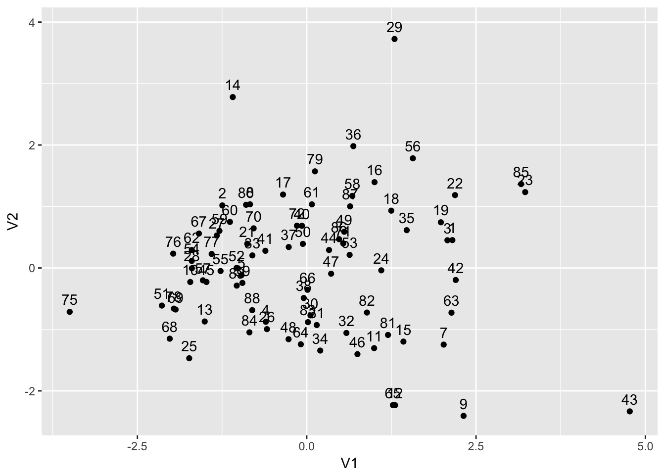
University of Chicago, Center for Spatial Data Science – anselin@uchicago.edu↩