Introduction
While there are many heuristics and algorithms to carry out contiguity-constrained clustering, the main one included in R is the SKATER approach from Assuncao et al (2006). This is implemented in the spdep package. The algorithm is based on pruning a minimum spanning tree constructed from the contiguity structure of the spatial units that need to be grouped.
Getting to the clusters involves several steps, including building a graph for the contiguity structure, computing the minimum spanning tree for that graph, and finally pruning the tree for the desired number of clusters.
In addition to the cluster algorithm, we will also explore some very rudimentary mapping functionality in R, using the rgdal and maptools packages, and the underlying spatial data structures from sp. We only apply the bare bones functionality, since an extensive treatment of mapping and GIS operations in R is beyond our scope. Also, mapping funtionality is a rapidly moving target in R and in some sense maptools is a bit old school, but it works.
We use readOGR to read the shape file Guerry_85.shp that contains observations on many of socio-economic characteristics for the 85 French departments.
Note: this is written with R beginners in mind, more seasoned R users can probably skip most of the comments on data structures and other R particulars.
Items covered:
reading a shape file and extracting data from a SpatialPolygonDataFrame
create a neighbor list object, e.g., using poly2nb or reading in a gal file
plot the neighbor list as a graph with the community area boundaries
compute a “distance” or “cost” between neighbors using nbcosts
create a binary list weight object using the just computed costs as the weights
use the weights object to construct a minimum spanning tree with mstree
plot the minimum spanning tree with the community area boundaries
apply the skater algorithm to obtain clusters
plot the pruned minimum spanning tree
map the clusters
Packages used:
rgdal
spdep
maptools
Preliminaries
Required libraries
library(rgdal)## Loading required package: sp## rgdal: version: 1.2-8, (SVN revision 663)
## Geospatial Data Abstraction Library extensions to R successfully loaded
## Loaded GDAL runtime: GDAL 2.1.3, released 2017/20/01
## Path to GDAL shared files: /Library/Frameworks/R.framework/Versions/3.4/Resources/library/rgdal/gdal
## Loaded PROJ.4 runtime: Rel. 4.9.3, 15 August 2016, [PJ_VERSION: 493]
## Path to PROJ.4 shared files: /Library/Frameworks/R.framework/Versions/3.4/Resources/library/rgdal/proj
## Linking to sp version: 1.2-4library(spdep)## Loading required package: Matrixlibrary(maptools)## Checking rgeos availability: TRUEReading shape file and extracting the data
We use the readOGR function from the rgdal package to read the shape file. This is now the preferred way to read a shape file (or any geographical layer supported) into R (the readShapePoly function from the maptools package also works, but will at some point become deprecated, so we no longer use it).
This creates a special data structure, called a SpatialPolygonDataFrame that contains both the spatial information (the coordinates of the polygon boundaries) as well as the actual data (attributes). The data are contained in the @data slot and need to be referred to as such. They can be converted to a non-spatial data frame using the data.frame command.
First, we read in the shape file. The readOGR function requires (at least) two arguments: the dsn and the layer. This may seem a bit confusing at first, but it allows for much greater flexibility in terms of data sources. The dsn refers to the folder where the spatial data reside. If your current working directory has all the files, the easiest way is to set it to “.” (the dot refers to the current working directory). The layer is the name of the shape file, but without the usual shp extension.
france <- readOGR(dsn=".",layer="Guerry_85")## OGR data source with driver: ESRI Shapefile
## Source: ".", layer: "Guerry_85"
## with 85 features
## It has 45 fields
## Integer64 fields read as strings: MainCty CL_CRMP CL_CRPROP CL_LIT CL_DON CL_Inf CL_SUIC BX_CRMP BX_CRMPROP BX_LIT BX_DON BX_INF BX_SUIC AREA_IDA summary shows the nature of the object as well as all the variables (your file may be slightly different).
summary(france)## Object of class SpatialPolygonsDataFrame
## Coordinates:
## min max
## x 47680 1031401
## y 1703258 2677441
## Is projected: TRUE
## proj4string :
## [+proj=lcc +lat_1=46.8 +lat_0=46.8 +lon_0=0 +k_0=0.99987742
## +x_0=600000 +y_0=2200000 +a=6378249.2 +b=6356514.999904194
## +pm=2.33722917 +units=m +no_defs]
## Data attributes:
## CODE_DE COUNT AVE_ID_ dept Region
## 01 : 1 Min. :1.000 Min. : 49 Min. : 1.00 C:17
## 02 : 1 1st Qu.:1.000 1st Qu.: 8612 1st Qu.:24.00 E:17
## 03 : 1 Median :1.000 Median :16732 Median :45.00 N:17
## 04 : 1 Mean :1.059 Mean :17701 Mean :45.08 S:17
## 05 : 1 3rd Qu.:1.000 3rd Qu.:26842 3rd Qu.:66.00 W:17
## 07 : 1 Max. :4.000 Max. :36521 Max. :89.00
## (Other):79
## Dprtmnt Crm_prs Crm_prp Litercy
## Ain : 1 Min. : 5883 Min. : 1368 Min. :12.00
## Aisne : 1 1st Qu.:14790 1st Qu.: 5990 1st Qu.:25.00
## Allier : 1 Median :18785 Median : 7624 Median :38.00
## Ardeche : 1 Mean :19961 Mean : 7881 Mean :39.14
## Ardennes: 1 3rd Qu.:26221 3rd Qu.: 9190 3rd Qu.:52.00
## Ariege : 1 Max. :37014 Max. :20235 Max. :74.00
## (Other) :79
## Donatns Infants Suicids MainCty Wealth
## Min. : 1246 Min. : 2660 Min. : 3460 1:10 Min. : 1.00
## 1st Qu.: 3446 1st Qu.:14281 1st Qu.: 15400 2:65 1st Qu.:22.00
## Median : 4964 Median :17044 Median : 26198 3:10 Median :44.00
## Mean : 6723 Mean :18983 Mean : 36517 Mean :43.58
## 3rd Qu.: 9242 3rd Qu.:21981 3rd Qu.: 45180 3rd Qu.:65.00
## Max. :27830 Max. :62486 Max. :163241 Max. :86.00
##
## Commerc Clergy Crm_prn Infntcd
## Min. : 1.00 Min. : 2.00 Min. : 1.00 Min. : 1
## 1st Qu.:21.00 1st Qu.:23.00 1st Qu.:22.00 1st Qu.:23
## Median :42.00 Median :44.00 Median :43.00 Median :44
## Mean :42.33 Mean :43.93 Mean :43.06 Mean :44
## 3rd Qu.:63.00 3rd Qu.:65.00 3rd Qu.:64.00 3rd Qu.:65
## Max. :86.00 Max. :86.00 Max. :86.00 Max. :86
##
## Dntn_cl Lottery Desertn Instrct
## Min. : 1.00 Min. : 1.00 Min. : 1.00 Min. : 1.00
## 1st Qu.:22.00 1st Qu.:22.00 1st Qu.:23.00 1st Qu.:23.00
## Median :43.00 Median :43.00 Median :44.00 Median :42.00
## Mean :43.02 Mean :43.04 Mean :43.91 Mean :43.34
## 3rd Qu.:64.00 3rd Qu.:64.00 3rd Qu.:65.00 3rd Qu.:65.00
## Max. :86.00 Max. :86.00 Max. :86.00 Max. :86.00
##
## Prsttts Distanc Area Pop1831 CL_CRMP
## Min. : 0.0 Min. : 0.0 Min. : 762 Min. :129.1 0:59
## 1st Qu.: 6.0 1st Qu.:119.7 1st Qu.: 5361 1st Qu.:283.8 1: 9
## Median : 34.0 Median :199.2 Median : 6040 Median :346.3 2:14
## Mean : 143.5 Mean :204.1 Mean : 6117 Mean :380.8 3: 3
## 3rd Qu.: 117.0 3rd Qu.:283.8 3rd Qu.: 6815 3rd Qu.:445.2
## Max. :4744.0 Max. :403.4 Max. :10000 Max. :989.9
##
## CL_CRPROP CL_LIT CL_DON CL_Inf CL_SUIC BX_CRMP BX_CRMPROP BX_LIT BX_DON
## 0:69 0:48 0:56 0:69 0:53 2:21 2:21 2:20 2:21
## 1: 6 1:17 1: 8 1: 7 1:13 3:21 3:21 3:22 3:21
## 2: 7 2:20 2:17 2: 6 2:17 4:22 4:22 4:22 4:22
## 3: 3 3: 2 3: 2 3: 2 5:21 5:18 5:21 5:19
## 4: 2 4: 1 6: 3 6: 2
##
##
## BX_INF BX_SUIC AREA_ID PC1 PC2
## 1: 1 2:21 1 : 1 Min. :-4.76964 Min. :-2.406826
## 2:20 3:21 10 : 1 1st Qu.:-0.99525 1st Qu.:-0.771465
## 3:21 4:22 11 : 1 Median : 0.05716 Median : 0.000518
## 4:22 5:16 12 : 1 Mean : 0.00000 Mean : 0.000000
## 5:16 6: 5 13 : 1 3rd Qu.: 1.09196 3rd Qu.: 0.644247
## 6: 5 14 : 1 Max. : 3.49999 Max. : 3.725174
## (Other):79
## PC3 PC4 PC5
## Min. :-3.138126 Min. :-2.73920 Min. :-1.312376
## 1st Qu.:-0.700550 1st Qu.:-0.40852 1st Qu.:-0.551329
## Median : 0.005259 Median : 0.04634 Median : 0.005071
## Mean : 0.000000 Mean : 0.00000 Mean : 0.000000
## 3rd Qu.: 0.802456 3rd Qu.: 0.50856 3rd Qu.: 0.383585
## Max. : 2.299306 Max. : 2.43883 Max. : 2.025063
##
## PC6
## Min. :-1.67472
## 1st Qu.:-0.31903
## Median :-0.01997
## Mean : 0.00000
## 3rd Qu.: 0.33713
## Max. : 1.42404
## We can create a simple map of the area boundaries using the plot command. We use one option to make the border lines a bit thinner and less bold (try the default if you are interested).
plot(france,border=gray(0.5))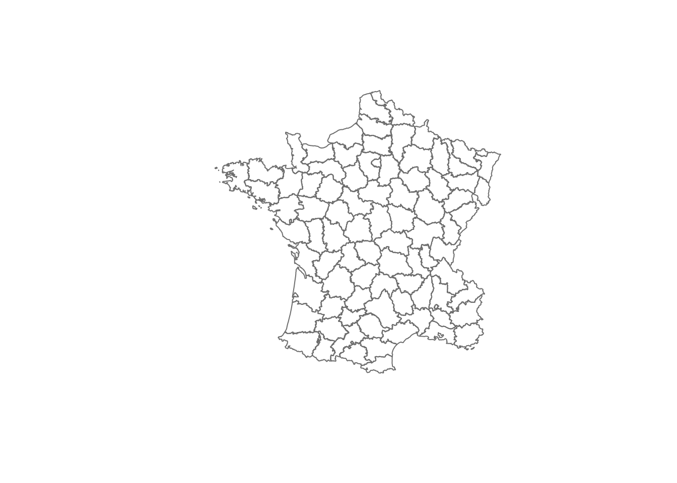
We first create a list with the desired variable names and then extract those using the @data slot and the standard bracketed subsetting (note the comma with the empty space before it to indicate that we want all the rows/observations). We use the same six variables as before.
vars <- c("Crm_prs","Crm_prp","Litercy","Donatns","Infants","Suicids")
dat <- data.frame(france@data[,vars])
summary(dat)
## Crm_prs Crm_prp Litercy Donatns
## Min. : 5883 Min. : 1368 Min. :12.00 Min. : 1246
## 1st Qu.:14790 1st Qu.: 5990 1st Qu.:25.00 1st Qu.: 3446
## Median :18785 Median : 7624 Median :38.00 Median : 4964
## Mean :19961 Mean : 7881 Mean :39.14 Mean : 6723
## 3rd Qu.:26221 3rd Qu.: 9190 3rd Qu.:52.00 3rd Qu.: 9242
## Max. :37014 Max. :20235 Max. :74.00 Max. :27830
## Infants Suicids
## Min. : 2660 Min. : 3460
## 1st Qu.:14281 1st Qu.: 15400
## Median :17044 Median : 26198
## Mean :18983 Mean : 36517
## 3rd Qu.:21981 3rd Qu.: 45180
## Max. :62486 Max. :163241Finally, as is customary, we standardize the variables using the scale function.
sdat <- scale(dat)
summary(sdat)
## Crm_prs Crm_prp Litercy Donatns
## Min. :-1.9287 Min. :-2.13649 Min. :-1.55677 Min. :-1.1263
## 1st Qu.:-0.7084 1st Qu.:-0.62039 1st Qu.:-0.81111 1st Qu.:-0.6739
## Median :-0.1611 Median :-0.08441 Median :-0.06546 Median :-0.3618
## Mean : 0.0000 Mean : 0.00000 Mean : 0.00000 Mean : 0.0000
## 3rd Qu.: 0.8576 3rd Qu.: 0.42926 3rd Qu.: 0.73756 3rd Qu.: 0.5179
## Max. : 2.3363 Max. : 4.05222 Max. : 1.99944 Max. : 4.3400
## Infants Suicids
## Min. :-1.8443 Min. :-1.0495
## 1st Qu.:-0.5313 1st Qu.:-0.6704
## Median :-0.2191 Median :-0.3276
## Mean : 0.0000 Mean : 0.0000
## 3rd Qu.: 0.3387 3rd Qu.: 0.2750
## Max. : 4.9153 Max. : 4.0232Neighbor list
We could read in the neighbor information from a GAL file, but to illustrate some of the functionality associated with the SpatialPolygonDataFrame data structure, we use the poly2nb function from spdep. We pass the name of the spatial polygons data frame to creates a neighbor list object, as indicated by the summary (see also the lab notes on spatial weights in spdep).
france.nb <- poly2nb(france)
summary(france.nb)
## Neighbour list object:
## Number of regions: 85
## Number of nonzero links: 420
## Percentage nonzero weights: 5.813149
## Average number of links: 4.941176
## Link number distribution:
##
## 2 3 4 5 6 7 8
## 7 11 12 16 30 7 2
## 7 least connected regions:
## 22 26 54 59 63 65 70 with 2 links
## 2 most connected regions:
## 46 72 with 8 linksAs we did in the treatment of spatial weights, we can draw a graph representation of the neighbor structure. Since we now can plot the community area boundaries as well, we plot this graph on top of the map. The first plot command gives the boundaries. This is followed by the plot of the neighbor list object, with coordinates applied to the original SpatialPolygonDataFrame (chicago) to extract the centroids of the polygons. These are used as the nodes for the graph representation. We also set the color to blue and specify add=TRUE to plot the network on top of the boundaries.
Note that if you plot the network first and then the boundaries, some of the areas will be clipped. This is because the plotting area is determined by the characteristics of the first plot. In this example, because the boundary map extends further than the graph, we plot it first.
plot(france,border=gray(.5))
plot(france.nb,coordinates(france),col="blue",add=TRUE)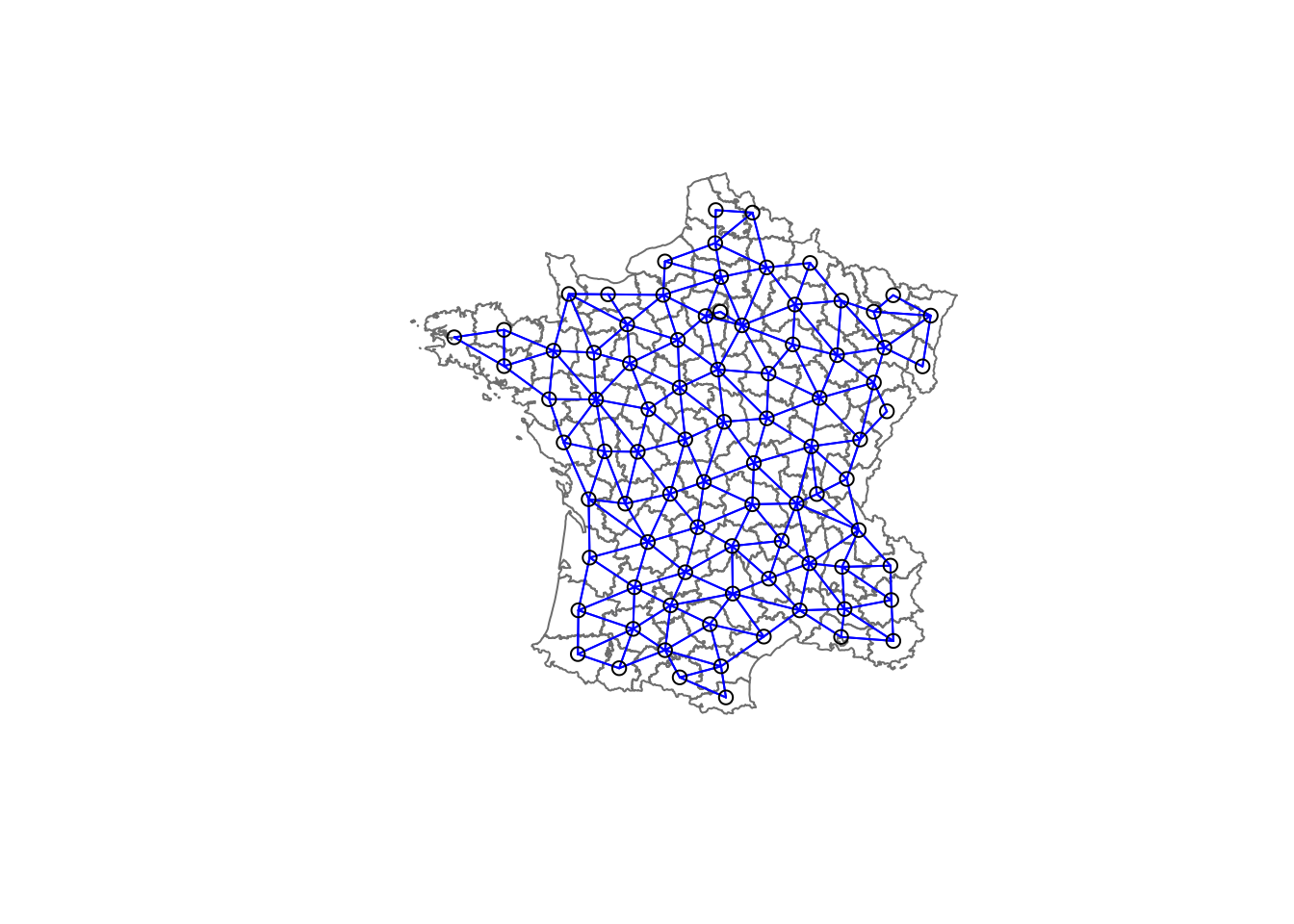
Minimum spanning tree
The skater algorithm works on a reduced search space determined by the minimum spanning tree (MST) for the observations. The MST is a graph that includes all the nodes in the network, but passes through each only once. So, it reduces the complexity of the original graph to one where each node is connected to only one other node. The resulting tree has n nodes and n-1 edges. The “minimum” part pertains to a cost function that is minimized. The objective is to minimize the overall length (or cost) of the tree. In its simplest form, the cost consists of the distances between the nodes. Here, however, a more general measure of cost is used in the form of the multivariate dissimilarity measure between each pair of nodes. This is based on a multivariate Euclidean distance between the standardized values for the variables, as was the case in the other clustering algorithms.
Edge costs
The first step in the process is to compute the costs associated with each edge in the neighbor list. In other words, for each observation, the dissimilarity is computed between it and each of its neighbors (as defined by the neighbor list). In the spdep package, this is carried out by the nbcosts function. Its arguments are the neighbor list and the standardized data frame (sdat in our example).
We check the first few items using the head command (a summary is not meaningful).
lcosts <- nbcosts(france.nb,sdat)
head(lcosts)## [[1]]
## [1] 3.726789 3.639887 5.262680 2.296905
##
## [[2]]
## [1] 2.0048994 1.9539965 0.9544817 0.9635145 0.9790028 1.4751302
##
## [[3]]
## [1] 3.286812 4.475697 3.085833 2.750602 2.555813 3.601231
##
## [[4]]
## [1] 1.7244481 0.8609304 1.7799800 1.0384114
##
## [[5]]
## [1] 1.724448 2.022424 2.749065
##
## [[6]]
## [1] 3.319378 2.198511 3.707139 3.014113 4.626438 2.735482 3.471025For each observation, this gives the pairwise dissimilarity between its values on the six variables and the values for the neighboring observations (from the neighbor list). Basically, this is the notion of a generalized weight for a spatial weights matrix. We therefore incorporate these costs into a weights object in the same way as we did in the calculation of inverse distance weights. In other words, we convert the neighbor list to a list weights object by specifying the just computed lcosts as the weights. We need to specify the style as B to make sure the cost values are not row-standardized.
france.w <- nb2listw(france.nb,lcosts,style="B")
summary(france.w)## Characteristics of weights list object:
## Neighbour list object:
## Number of regions: 85
## Number of nonzero links: 420
## Percentage nonzero weights: 5.813149
## Average number of links: 4.941176
## Link number distribution:
##
##  2  3  4  5  6  7  8
##  7 11 12 16 30  7  2
## 7 least connected regions:
## 22 26 54 59 63 65 70 with 2 links
## 2 most connected regions:
## 46 72 with 8 links
##
## Weights style: B
## Weights constants summary:
## n nn S0 S1 S2
## B 85 7225 979.5928 5550.898 53659.74Minimum spanning tree
The mininum spanning tree is computed by means of the mstree function from the spdep package. The only required argument is the weights object. We pass the just created france.w weights list. The result is a special type of matrix. It summarizes the tree by giving each edge as the pair of connected nodes, followed by the cost associated with that edge.
After computing the MST, we check its class, dimension and show the first few elements.
france.mst <- mstree(france.w)
class(france.mst)
## [1] "mst" "matrix"dim(france.mst)## [1] 84 3Note that the dimension is 84 and not 85, since the minimum spanning tree consists of n-1 edges (links) needed to traverse all the nodes.
head(france.mst)## [,1] [,2] [,3]
## [1,] 4 24 0.8609304
## [2,] 24 80 0.8152341
## [3,] 80 12 0.9962710
## [4,] 24 36 1.2545273
## [5,] 80 79 1.5507884
## [6,] 80 28 1.5508092The plot method for the MST includes a way to show the observation numbers of the nodes in addition to the edges. As before, we plot this together with the departmental boundaries. We can see how the initial neighbor list is simplified to just one edge connecting each of the nodes, while passing through all the nodes.
plot(france.mst,coordinates(france),col="blue",
      cex.lab=0.7)
plot(france,border=gray(.5),add=TRUE)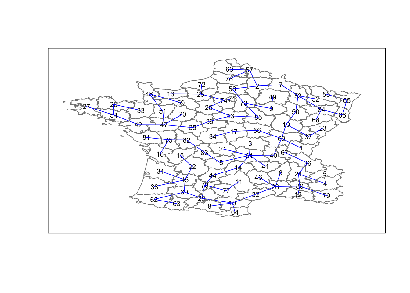
Contiguity-constrained cluster
The skater function takes three mandatory arguments: the first two columns of the MST matrix (i.e., not the costs), the standardized data matrix (to update the costs as units are being grouped), and the number of cuts. The latter is possibly somewhat confusingly set to one less than the number of clusters. So, the value specified is not the number of clusters, but the number of cuts in the graph, one less than the number of clusters.
The skater function has several additional options, but we will not pursue those further here.
The result of the skater function is an object of class skater. We examine its contents using str (the summary command is not meaningful).
k = 4
To obtain four clusters, we specify the first two columns of the minimum spanning tree matrix, the data frame with the standardized values (sdat), and set the number of cuts to 3.
clus4 <- skater(france.mst[,1:2],sdat,3)
str(clus4)
## List of 8
## $ groups : num [1:85] 4 2 4 1 1 1 2 1 2 1 ...
## $ edges.groups:List of 4
## ..$ :List of 3
## .. ..$ node: num [1:29] 14 44 32 28 78 10 80 29 62 24 ...
## .. ..$ edge: num [1:28, 1:3] 32 28 80 62 10 10 30 28 22 29 ...
## .. ..$ ssw : num 51.2
## ..$ :List of 3
## .. ..$ node: num [1:28] 43 85 73 7 53 25 84 58 2 26 ...
## .. ..$ edge: num [1:27, 1:3] 25 7 84 53 58 85 50 26 73 2 ...
## .. ..$ ssw : num 44.4
## ..$ :List of 3
## .. ..$ node: num [1:12] 39 35 42 47 54 20 51 48 27 33 ...
## .. ..$ edge: num [1:11, 1:3] 42 47 54 54 20 35 47 51 39 47 ...
## .. ..$ ssw : num 21.6
## ..$ :List of 3
## .. ..$ node: num [1:16] 61 18 75 83 40 82 69 17 56 81 ...
## .. ..$ edge: num [1:15, 1:3] 18 61 61 83 75 61 82 69 61 61 ...
## .. ..$ ssw : num 39.5
## $ not.prune : NULL
## $ candidates : int [1:4] 1 2 3 4
## $ ssto : num 192
## $ ssw : num [1:4] 192 176 165 157
## $ crit : num [1:2] 1 Inf
## $ vec.crit : num [1:85] 1 1 1 1 1 1 1 1 1 1 ...
## - attr(*, "class")= chr "skater"The most interesting component of this list structure is the groups vector containing the labels of the cluster to which each observation belongs (as before, the label itself is arbitrary). This is followed by a detailed summary for each of the clusters in the edges.groups list. Sum of squares measures are given as ssto for the total and ssw to show the effect of each of the cuts on the overall criterion.
We check the cluster assignment.
ccs4 <- clus4$groups
ccs4
## [1] 4 2 4 1 1 1 2 1 2 1 1 1 2 1 1 4 4 4 2 3 4 1 2 1 2 2 3 1 1 1 1 1 3 4 3
## [36] 1 2 1 3 4 4 3 2 1 1 1 3 3 2 2 3 2 2 3 2 4 2 2 3 2 4 1 1 1 2 2 1 2 4 3
## [71] 2 2 2 2 4 2 1 1 1 1 4 4 4 2 2We can find out how many observations are in each cluster by means of the table command. Parenthetially, we can also find this as the dimension of each vector in the lists contained in edges.groups. For example, the first list has node with dimension 12, which is also the number of observations in the first cluster.
table(ccs4)## ccs4
## 1 2 3 4
## 29 28 12 16We can now also plot the pruned tree that shows the four clusters on top of the community area boundaries, using the same logic as before. We set each group (groups in the cluster object) to a different color.
plot(clus4,coordinates(france),cex.lab=.7,
    groups.colors=c("red","green","blue","brown"))
plot(france,border=gray(.5),add=TRUE)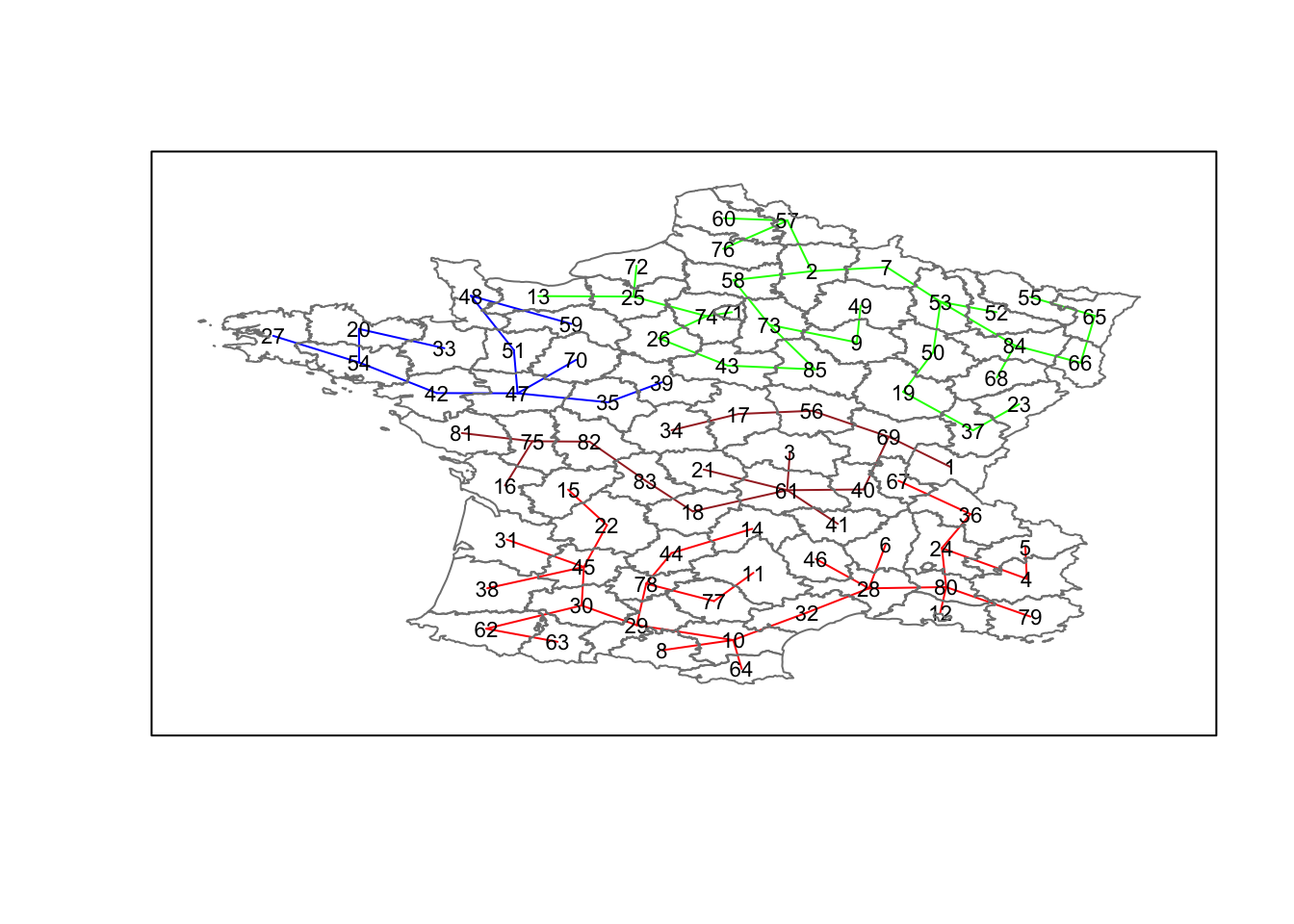
Finally, to illustrate this in a map, we can create a unique values map by plotting the france object and specifying the variable clus4.groups in brackets. It’s not pretty, but it works.
plot(france,col=c("red","green","blue","brown")[clus4$groups])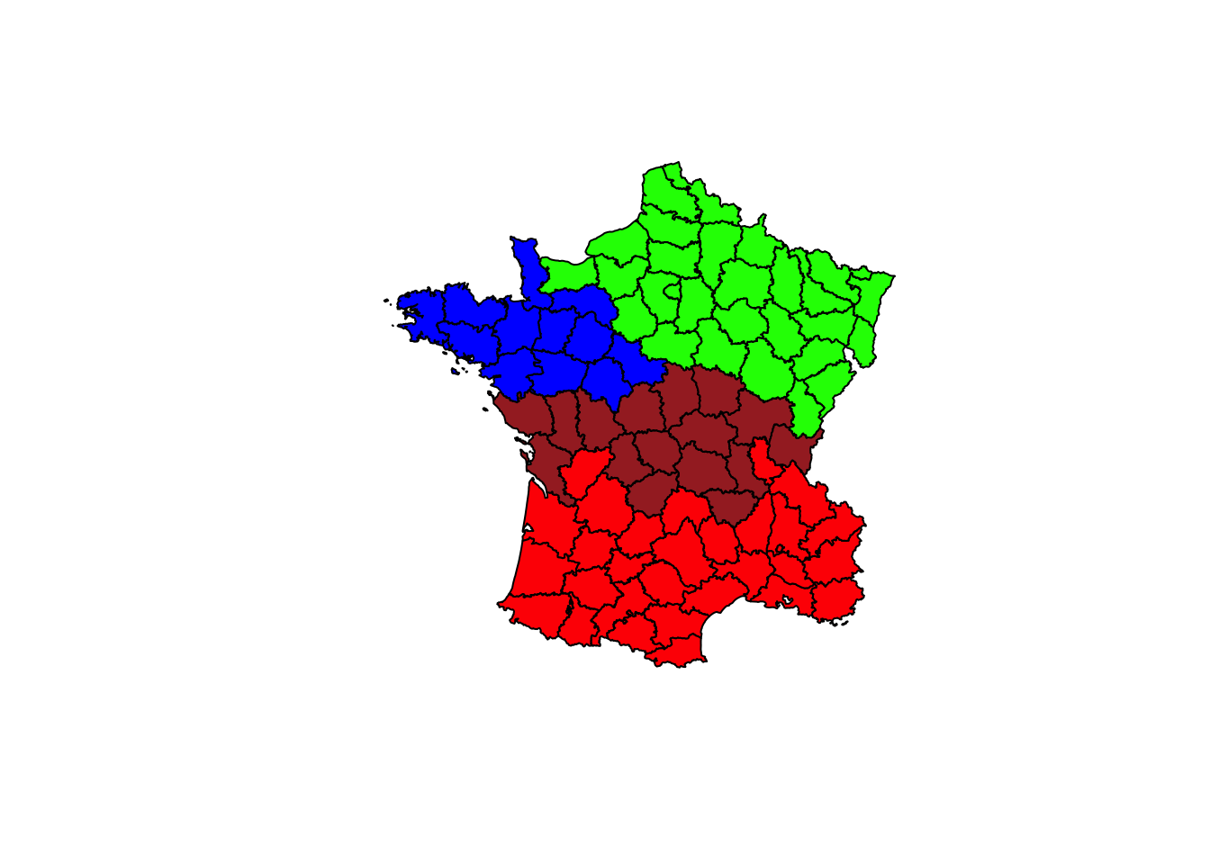
k = 6
We repeat the process, but now specify 5 as the number of cuts, which will yield six clusters. We only show the output.
clus6 <- skater(france.mst[,1:2],sdat,5)
ccs6 <- clus6$groups
ccs6
## [1] 4 2 4 1 1 1 2 1 2 1 1 1 2 1 1 6 4 4 2 5 4 1 2 1 2 2 5 1 1 1 1 1 5 4 3
## [36] 1 2 1 3 4 4 3 2 1 1 1 3 3 2 2 3 2 2 5 2 4 2 2 3 2 4 1 1 1 2 2 1 2 4 3
## [71] 2 2 2 2 6 2 1 1 1 1 6 6 6 2 2table(ccs6)## ccs6
## 1 2 3 4 5 6
## 29 28 8 11 4 5plot(clus6,coordinates(france),cex.lab=.7,
groups.colors=c("red","green","blue","brown","gray","yellow"))
plot(france,border=gray(.5),add=TRUE)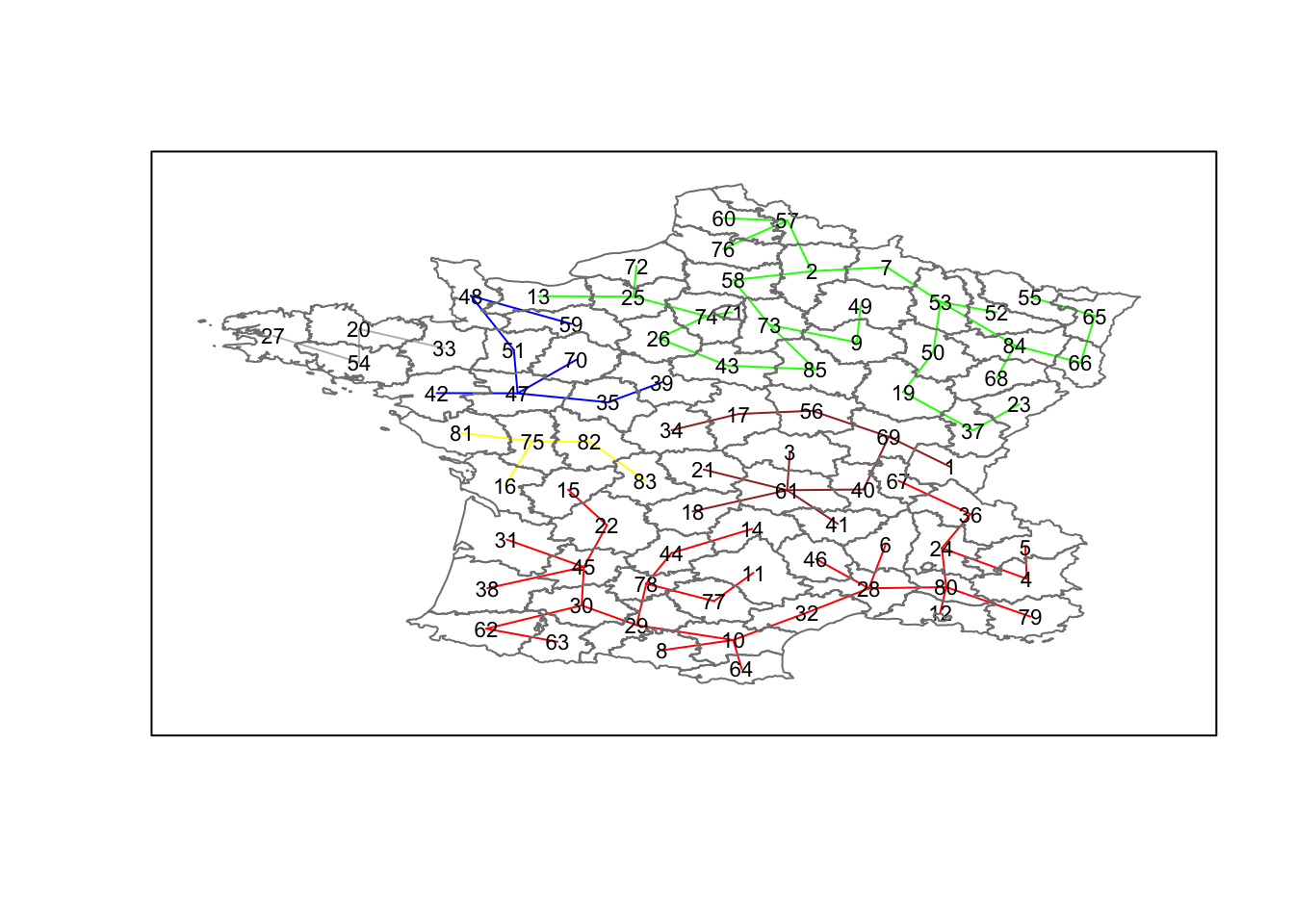
plot(france,col=c("red","green","blue","brown","gray","yellow")[clus6$groups])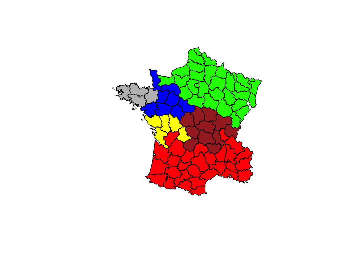
In order to include the cluster information in the GeoDa exploratory framework, we can proceed in the usual fashion by creating a data frame with the cluster labels, adding an ID for the community areas and writing this out to a csv file.
University of Chicago, Center for Spatial Data Science – anselin@uchicago.edu↩