Exploratory Data Analysis (1)

Univariate and Bivariate Analysis

Introduction

In this Chapter, we will begin to explore the EDA functionality in GeoDa, in particular the methods that deal with one or two variables. We leave the treatment of multiple variables for the next Chapter. We also illustrate the powerful linking and brushing capability that is central to the architecture of the program. We start with the description and visualization of a single variable, and then move on to the bivariate scatter plot and an exploration of spatial heterogeneity.

We will again use a data set with demographic and socio-economic information for 55 New York City sub-boroughs.

Objectives

• Computing descriptive statistics and creating visualizations of the distribution of a single variable (histogram, box plot)

• Interpreting a scatter plot and scatter plot smoothing (LOWESS)

• Carrying out scatter plot brushing and linking

• Assessing spatial heterogeneity by means of the Averages Chart

• Assessing spatial heterogeneity through the Chow test

GeoDa functions covered

• Linking and brushing graphs and maps
• Variable settings dialog
• Explore > Histogram
  • Choose Intervals option
  • Histogram Classification option
  • View > Set as Unique Value
  • View > Display Statistics option
• Explore > Box Plot
  • Hinge option
• Explore > Scatter Plot
  • View > Display Precision option
  • Data option
  • Smoother option
  • LOWESS parameters setting
  • Regimes Regression option and Chow test
• Explore > Averages Chart

Preliminaries

We will continue to illustrate the various operations by means of the data set with demographic and socio-economic information for 55 New York City sub-boroughs that comes built-in with GeoDa. It is also contained in the GeoDa Center data set collection.

• nyc: socio-economic data for 55 New York City sub-boroughs

As before, since the data set is built-in, there is no real need to download the sample data, although it is useful in order to preserve any changes. Also, if earlier you created a project file to contain the custom map classification, you should load this gda file instead.

We will focus our attention on the functionality of the Explore menu, listed in Figure 1.

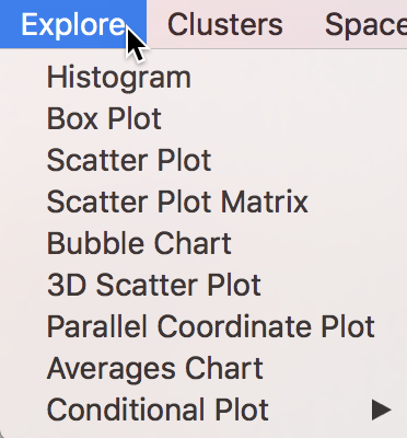
Figure 1: Explore menu items

The counterpart to the menu items are the collection of eight icons on the main toolbar, shown in Figure 2. The icon for the Averages Chart is separate, and is considered further below.

Figure 2: Explore toolbar icons

The first two icons on the left pertain to univariate analyses, respectively the Histogram and Box Plot. The Scatter Plot extends this to bivariate association. The other icons pertain to the analysis of multiple variables, which we leave to the next Chapter to consider.

Analyzing the Distribution of a Single Variable

Histogram

We begin our analysis with the simple description of the distribution of a single variable. Arguably the most familiar statistical graphic is the histogram, which is a discrete representation of the density function of a variable. In essence, the range of the variable (the difference between maximum and minimum) is divided into a number of equal intervals (or bins), and the number of observations that fall within each bin is depicted in a bar graph.

The histogram functionality is started by selecting Explore > Histogram from the menu, or by clicking on the Histogram toolbar icon, the left-most icon in the set in Figure 2.

This brings up the Variable Settings dialog, which lists all the numeric variables in the data set (string variables cannot be analyzed). Scroll down the list as in Figure 3 until you can select kids2000, the percentage of households with kids under age 18 in 2000. This is the same variable we used to illustrate some of the mapping functionality.

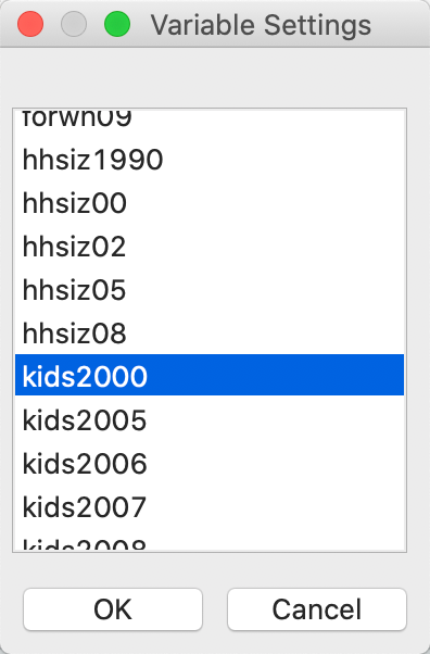
Figure 3: Histogram variable selection

After clicking OK, the default histogram appears, showing the distribution of the 55 observations over seven bins, as in Figure 4. Interestingly, we find that the second bin lacks observations, suggesting that a different set of intervals may be more appropriate.

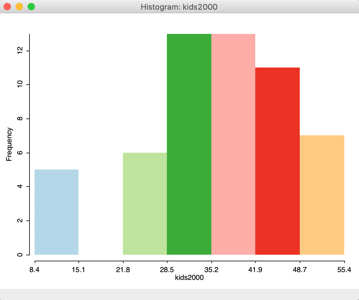
Figure 4: Default histogram

There are a number of important options for the histogram. Arguably the most important one is to set the number of bins or, alternatively, the values for the cut points.

The histogram options shown in Figure 5 are brought up in the usual fashion, by right clicking on the graph.

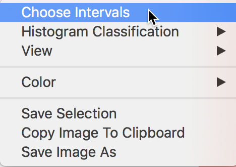
Figure 5: Choose intervals histogram option

Selecting the number of histogram bins

The Choose Intervals option, shown in Figure 5, allows for the customization of the number of bins in the histogram. A dialog appears that lets you set this value explicitly. The default is 7, but in our example, we change this to 5, as in Figure 6.

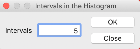
Figure 6: Histogram intervals set to 5

The resulting histogram now has five bars, as in Figure 7.

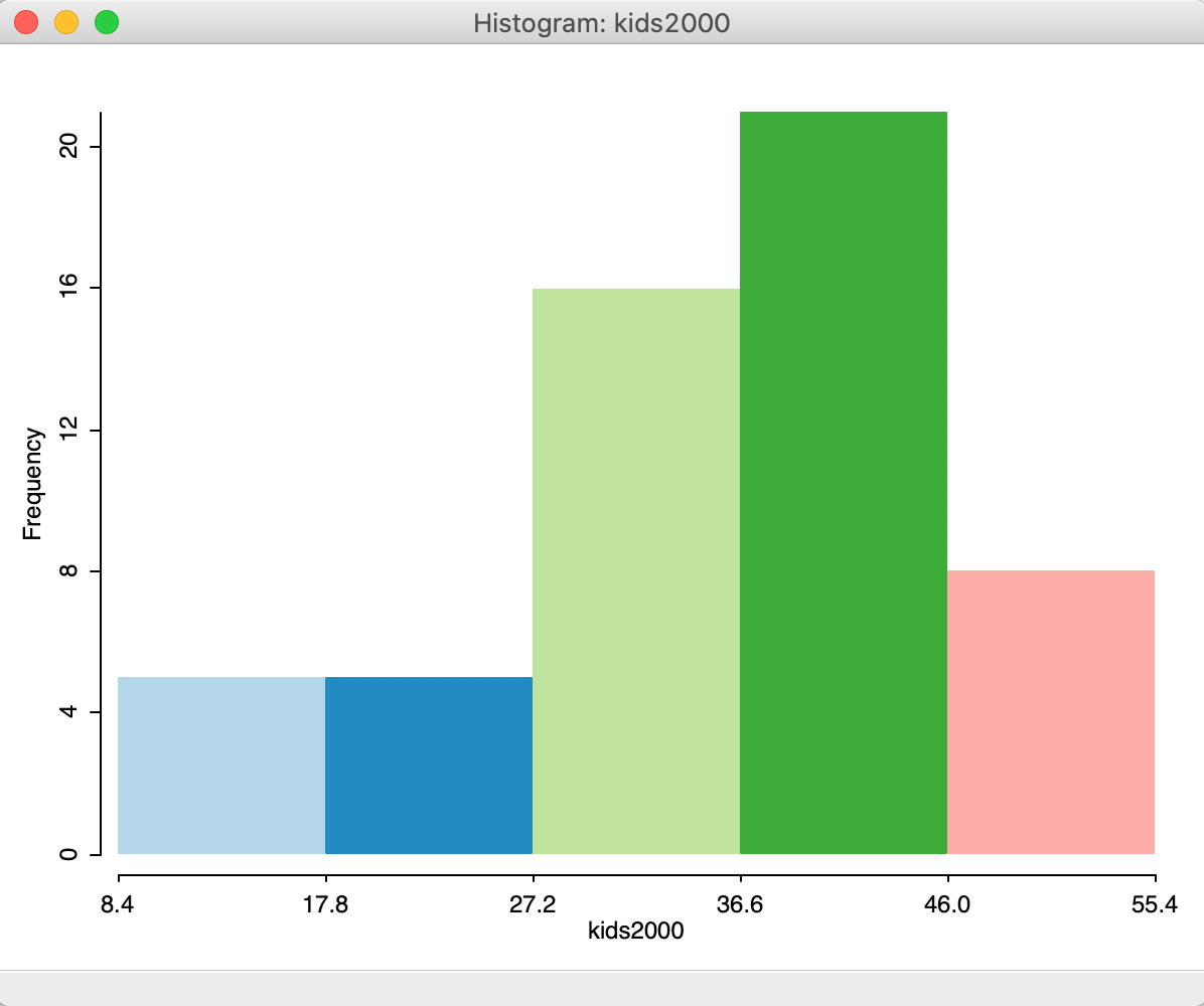
Figure 7: Histogram with 5 intervals

This takes care of the problem of the bin with missing observations.

Using a custom classification

Recall how we created a custom map classification based on the range of values for kids2000, and labeled it custom1. If you have loaded the project file with the NYC data, then this custom classification will be listed as an option for Histogram Classification, as shown in Figure 8. If you started from scratch, you will have to recreate the custom classification (for specifics, see the mapping chapter).

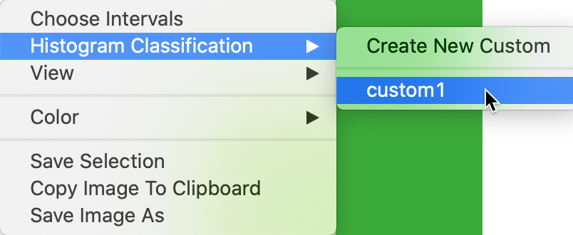
Figure 8: Selecting a custom histogram classification

The custom classification is the way GeoDa allows for cut points to be specified, instead of the number of bins. With custom1 selected, the histogram takes the form as in Figure 9, with six bins, as defined by this classification. The histogram has the exact same shape as the one portrayed in the Category Editor interface when creating these custom categories.

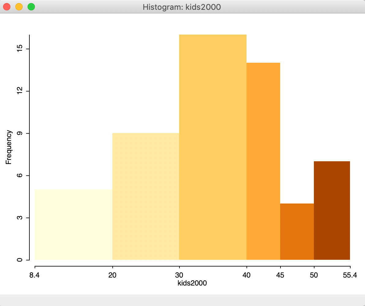
Figure 9: Histogram with custom intervals

Histograms for categorical variables

The default logic behind the histogram is to consider the range of the variable of interest (max - min) and compute the cut points based on the specified number of bins. For categorical variables, this leads to undesirable results.

To illustrate this, we create a map for kids2000 with the custom1 categories, and use Save Categories to create a categorical variable (say catkid20) for this classification.² The default histogram for this variable is as in Figure 10, clearly not something that reflects the discrete integer values associated with the categories. Rather, the cut points are based on the range of 5, divided by the default number of bins of 7, or a bin width of approximately 0.7. Indeed, the first bin goes from 1 to 1.7.

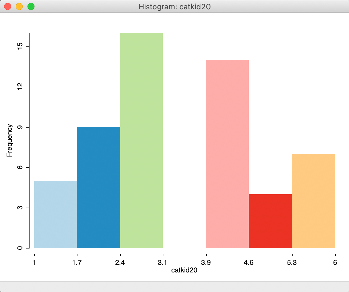
Figure 10: Default histogram for categorical variables

The View option of the histogram provides a way to deal with categorical variables by means of the Set as Unique Value item, shown in Figure 11. This option recognizes the discrete nature of the categorical variable and adjusts the cut point accordingly.

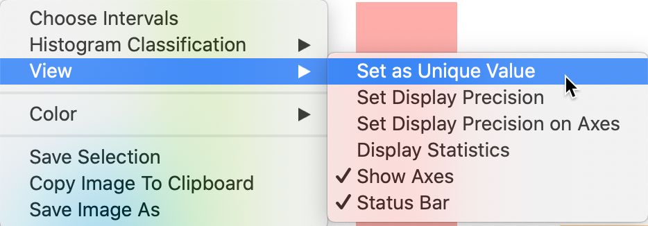
Figure 11: Selecting a unique value histogram classification

The result is shown in Figure 12, with six categories each associated with an identifying integer value.

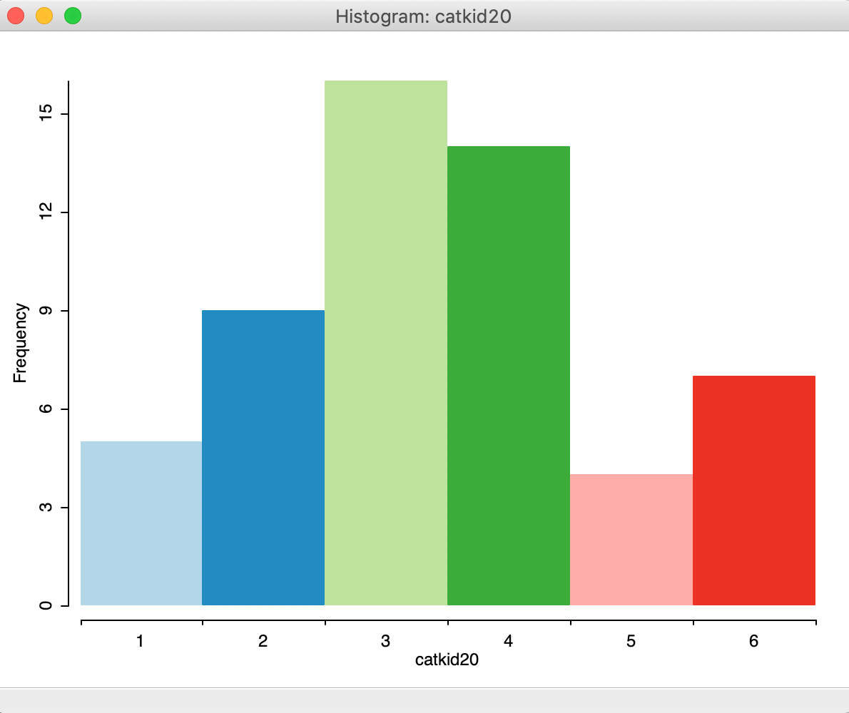
Figure 12: Unique value histogram for categorical variables

Display histogram statistics

An important option for the histogram (and any other statistical graph) is to be able to display descriptive statistics for the variable of interest. This is accomplished by selecting Display Statistics in the View option for the histogram (see Figure 11)

This option adds a number of descriptors below the graph. The summary statistics are given at the bottom, illustrated in Figure 13 for kids2000 with custom categories. We see that the 55 observations have a minimum value of 8.3815, a maximum of 55.3666, median of 38.2278, mean of 36.04 and a standard deviation of 11.2881. In addition, for the histogram, descriptive statistics are provided for each interval, showing the range for the interval, the number of observations as a count and as a percentage of the total number of observations, and the number of standard deviations away from the mean for the center of the bin. This allows us to identify potential outliers, e.g., as defined by those observations more than two standard deviations from the mean. In our example, no category satisfies this criterion.

The summary characteristics for a given bin also appear in the status bar when the cursor is moved over the corresponding bar. This works whether the descriptive statistics option is on or not. In our example in Figure 13, the cursor is over the fourth category.

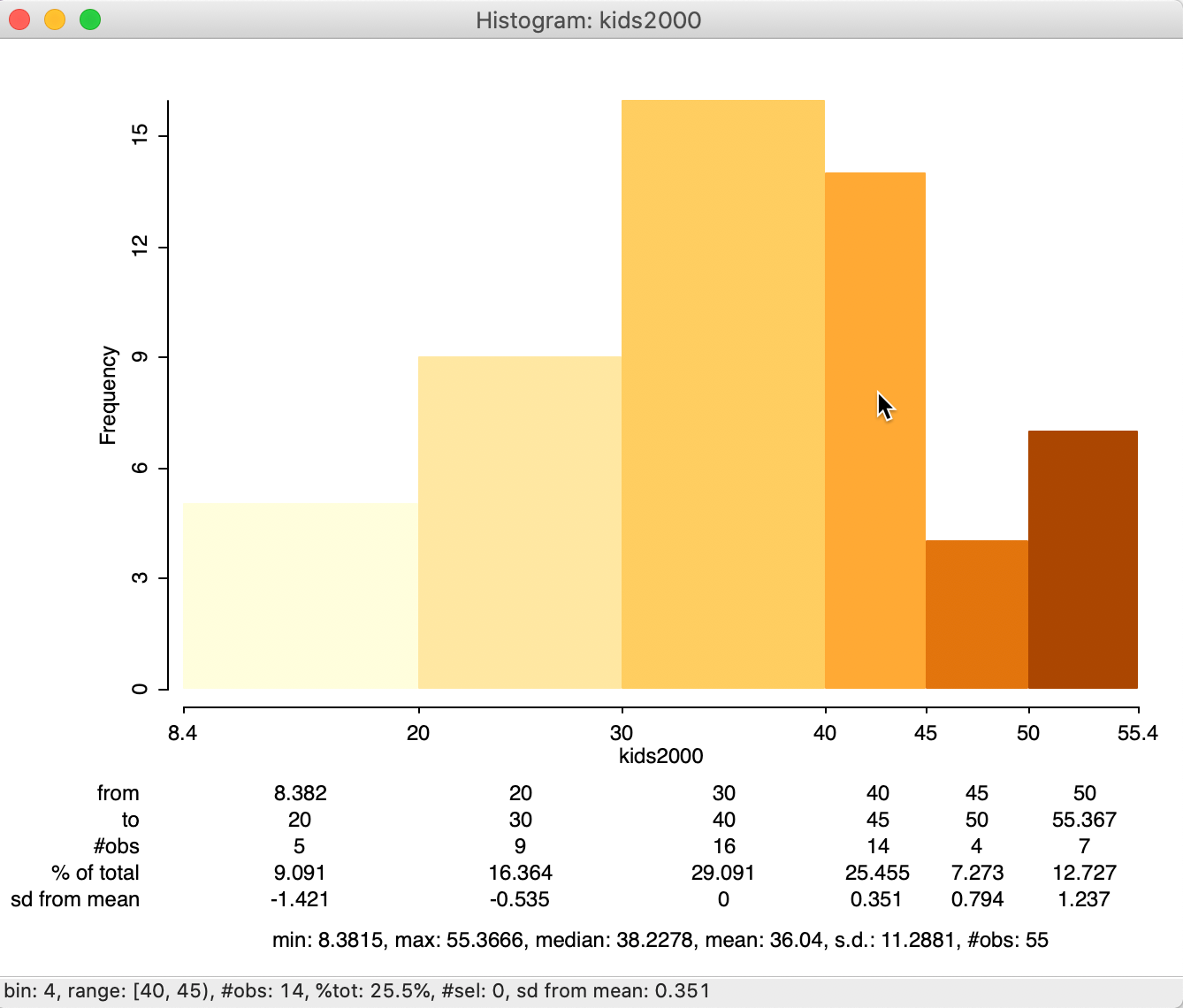
Figure 13: Histogram with descriptive statistics

Other histogram options

Other items available in the View option include customizing the precision of the axes and displayed statistics, respectively through View > Set Display Precision on Axes and View > Set Display Precision.

In addition, standard options for the histogram include adjustments to various color settings (Color), saving the selection (similar to what we saw for the map functionality), Copy the Image to Clipboard and saving the graph as an image file (again, identical to the map functionality).

Linking a histogram and a map

To illustrate the concept of linked graphs and maps, we continue with the custom histogram and make sure the default themeless map is available. When we select the two right-most bars in the histogram (click and shift-click to expand the selection), the highlighted bars keep their color, whereas the non-selected ones become transparent, as in the right-hand graph in Figure 14. This is the standard approach to visualize a selection in a graph in GeoDa.³

Immediately upon selection of the bars in the graph, the corresponding observations in the map are also highlighted, as in the left-hand graph in Figure 14. In our current example, the map is a simple themeless map (all areal units are green), but in more realistic applications, the map can be any type of choropleth map, for the same variable or for a different variable. The latter can be very useful in the exploration of categorical overlap between variables.

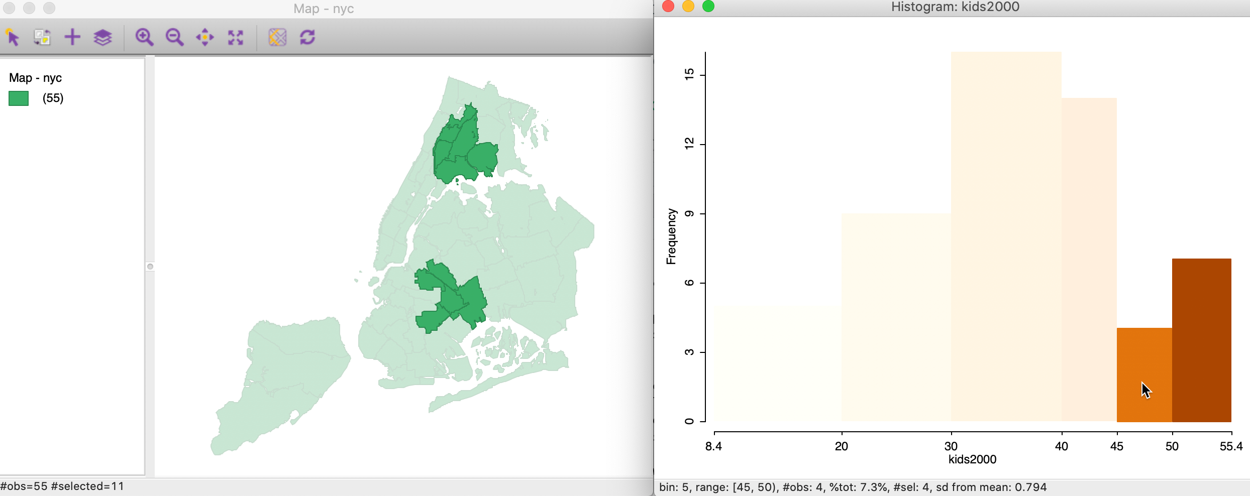
Figure 14: Linking a histogram and a map

The reverse linking works as well. For example, using a rectangular selection tool on the themeless map, we can select sub-boroughs in Manhattan and adjoining Brooklyn, as in the map in Figure 15. The linked histogram (right-hand graph in Figure 15) will show the attribute distribution for the selected spatial units as highlighted fractions of the bars (the transparent bars correspond to the unselected areal units).

In practice, we will be interested in assessing the extent to which the distribution of the selected observations (e.g., a sub-region) matches the overall distribution. When it does not, this may reveal the presence of spatial heterogeneity, to which we return below.

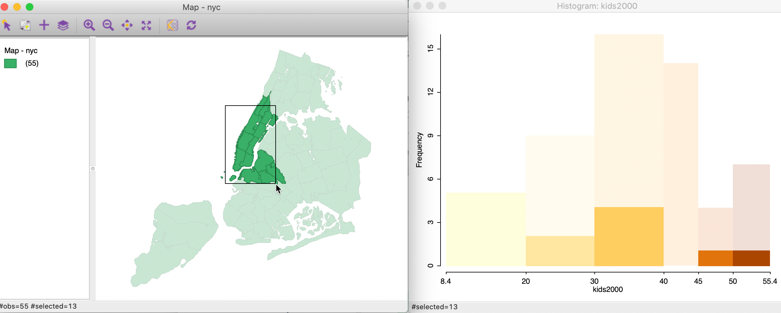
Figure 15: Linking a map and a histogram

As we have seen before, it is also possible to save the selection in the form of a 0-1 indicator variable with the Save Selection option.

The technique of linking, and its dynamic counterpart of brushing (more later) is central to the data exploration philosophy that is behind GeoDa (for a more elaborate exposition of the philosophy behind GeoDa, see Anselin, Syabri, and Kho 2006).

Box Plot

A box plot is an alternative visualization of the distribution of a single variable. It is invoked as Explore > Box Plot, or by selecting the Box Plot as the second icon from the left in the toolbar, shown in Figure 2.

Identical to the approach followed for the histogram, next appears a Variable Settings dialog to select the variable. In GeoDa, the default is that the variable from any previous analysis is already selected. In our example, we change this to the variable rent2008, which we already encountered in the illustration of the box map in the mapping Chapter.

The box plot for rent2008 is shown in Figure 16 (make sure to turn off any previous selection of observations).

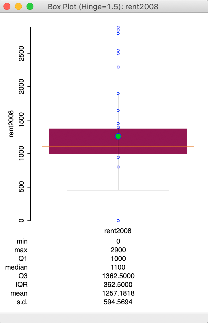
Figure 16: Default box plot

The box plot focuses on the quartiles of the distribution. The data points are sorted from small to large. The median (50 percent point) is represented by the horizontal orange bar in the middle of the distribution. The green dot above corresponds with the mean.

The brown rectangle goes from the first quartile (25th percentile) to the third quartile (75th percentile). The difference between the values that correspond to the third (1362.5) and the first quartile (1000) is referred to as the inter-quartile range (IQR). The inter-quartile range is a measure of the spread of the distribution, a non-parametric counterpart to the standard deviation. In our example, the IQR is 362.5 (1362.5 - 1000).

The horizontal lines drawn at the top and bottom of the graph are the so-called fences or hinges. They correspond to the values of the first quartile less 1.5xIQR (i.e., roughly 1000 - 362.5x1.5 = 275), and the third quartile plus 1.5xIQR (i.e., roughly 1362.5 + 362.5x1.5 = 2087.5). Observations that fall outside the fences are considered to be outliers.⁴

In our example in Figure 16, we have a single lower outlier value (corresponding to three observations), and six upper outlier observations. Note that the lower outliers are the observations that correspond with a value of 0 (the minimum), which we earlier had flagged as potentially suspicious. The outlier detection would seem to confirm this. Checking for strange values that may possibly be coding errors or suggest other measurement problems is one of the very useful applications of a box plot.

Box plot options

The default in GeoDa is to list the summary statistics at the bottom of the box plot. As was the case for the histogram, the statistics include the minimum, maximum, mean, median and standard deviation. In addition, the values for the first and third quartile and the resulting IQR are given as well. The listing of descriptive statistics can be turned off by unchecking View > Display Statistics (i.e., the default is the reverse of what held for the histogram, where the statistics had to be invoked explicitly).

The typical multiplier for the IQR to determine outliers is 1.5 (roughly equivalent to the practice of using two standard deviations in a parametric setting). However, a value of 3.0 is fairly common as well, which considers only truly extreme observations as outliers. The multiplier to determine the fence can be changed with the Hinge > 3.0 option (right click in the plot to select the options menu, and then choose the hinge value, as in Figure 17).

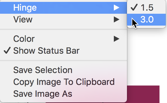
Figure 17: Change the box plot hinge

The resulting box plot, shown in Figure 18, no longer characterizes the lowest value as an outlier.

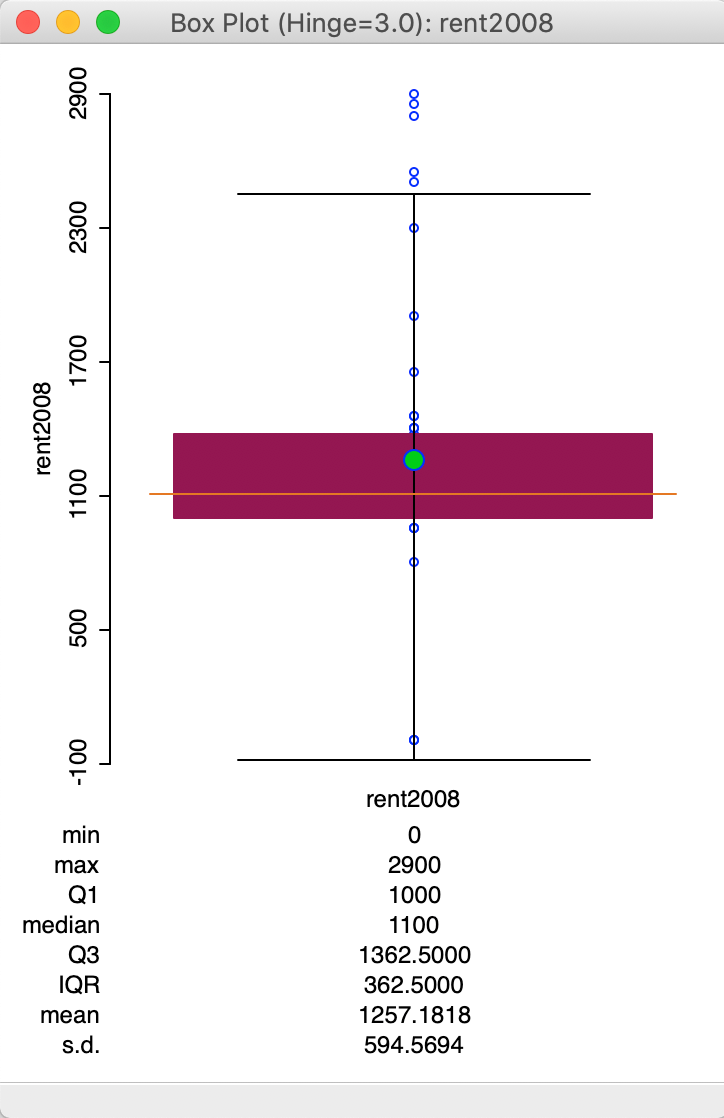
Figure 18: Box plot with hinge = 3.0

The other options for the box plot can be seen in Figure 17. Except for the Hinge option, these are the same as for the histogram, and are not further considered here.

Also, as is the case for any graph in GeoDa, linking and brushing are implemented, as already illustrated in the mapping Chapter.

The main purpose of the box plot in an exploratory strategy is to identify outlier observations. We have already seen how that is implemented in the idea of a box map to show whether such outliers also coincide in space. In later Chapters, we will cover more formal methods to assess such patterns.

Bivariate Analysis: The Scatter Plot

Scatter Plot basics

Default settings

The standard tool to assess a linear relationship between two variables is the scatter plot, a diagram with two axes, each corresponding to one of the variables. The observation (x, y) pairs are plotted as points in the diagram.

We create a scatter plot by selecting Explore > Scatter Plot from the menu, or by clicking on the matching toolbar icon, the third from the left in the EDA group on the toolbar, shown in Figure 2.

This brings up the Scatter Plot Variables dialog, where the variables for the X and Y axes need to be selected. In our example, illustrated in Figure 19, we will choose the percentage of households with kids under age 18 in 2000 (kids2000) as the X-variable, and the percentage of households receiving public assistance (pubast00) as the Y-variable.

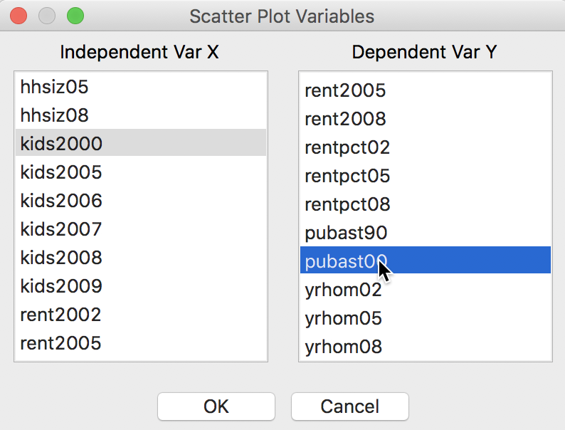
Figure 19: Scatter Plot variable selection

Clicking OK brings up the scatter plot, shown in 20.

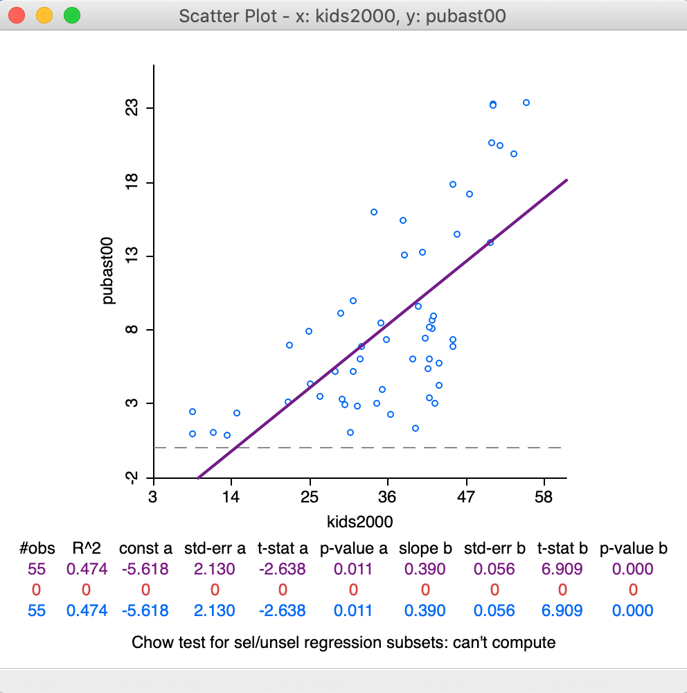
Figure 20: Default Scatter Plot

The default view of the scatter plot is to use the variables in their original scales (i.e., not standardized), show the axes through zero (as dashed lines), and fit a linear smoother (i.e., a least squares regression fit). In our example in Figure 20, there is only a horizontal axis, since all the x values are larger than zero.

In addition, at the bottom of the graph, several summary statistics are listed for the regression line. This includes the R² of the fit, and the estimate, standard error, t-statistic and p-value for both the intercept and the slope coefficient.

In the current setup, no observations are selected, so that the second line in the statistical summary in Figure 20 (all red zeros) has no values. This line pertains to the selected observations. The blue line at the bottom relates to the unselected observation. The sum of the number of observations in each of the two subsets always equals the total number of observations, listed on the top line. The three lines are listed because of the default View setting of Regimes Regression, even though there is currently no active selection (see also below).

Scatter Plot options

The scatter plot has several interesting options, many of which are listed in Figure 21, with a focus on the View items. As usual, the list of options is brought up by right clicking in the graph window or by selecting Options in the menu.

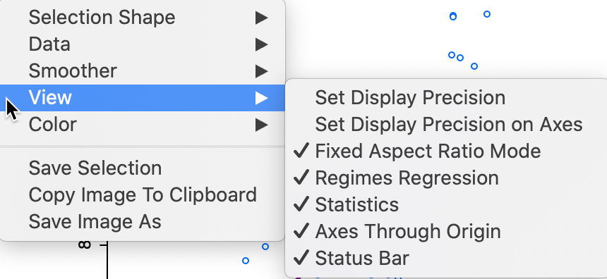
Figure 21: Scatter Plot options

The View option shows the default settings with the Statistics displayed below the graph, the Axes Through Origin shown as dashed lines, and the Status Bar active. Two other default settings are to have a Fixed Aspect Ratio and Regimes Regression active. When some observations are selected, the regimes regression setting will result in the computation of three different linear smoothers. We revisit this when we consider brushing the scatter plot.

Several of the other options should by now be familiar, such as the Selection Shape, Color, Save Selection and the two ways to save the image. In addition, as before, we can set the precision for the axes and the display itself. We do not further discuss these options again.

Correlation

The Data option provides a choice between the variables on their original scale (the default) and the use of standardized variables. Note that when you use the standardized form, by means of Data > View Standardized Data, the slope of the linear smoother (0.688) is also the correlation coefficient between the two variables, as in Figure 22. In all other respects, the look of the scatter plot is the same as before.

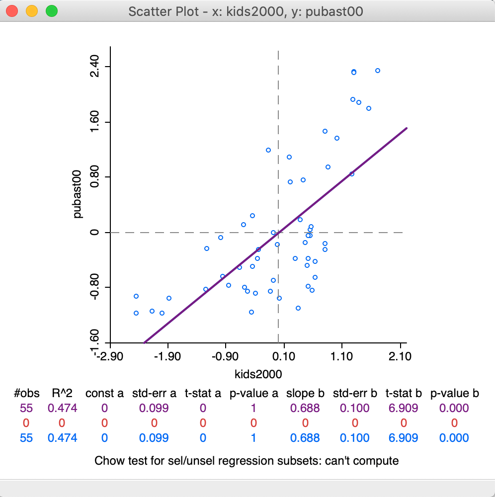
Figure 22: Scatter Plot for standardized values – correlation

Smoothing the scatter plot

The default setting is to implement a linear regression fit to the scatter plot points. An alternative that is better at exploring local nonlinearities is a so-called local regression fit. A local regression fit is a nonlinear procedure that computes the slope from a subset of observations on a small interval on the X-axis. In addition, values further removed from the center of the interval may be weighted down (similar to a kernel smoother). As the interval (the bandwidth) moves over the full range of observations, the different slopes are combined into a smooth curve (for a detailed overview of the methodological issues, see, e.g., Cleveland 1979; and Loader 1999, 2004).

A nonlinear local regression fit reveals potential nonlinearities in the bivariate relationship and may suggest the presence of structural breaks. Two common implementations are LOWESS, locally weighted scatter plot smoother, and LOESS, a local polynomial regression (the two are often confused, but implement different fitting algorithms).

In GeoDa, LOWESS is implemented. It is selected in the Smoother option, as shown in Figure 23.

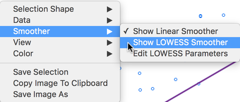
Figure 23: Scatter Plot smoothing options

Selecting the Show LOWESS Smoother option adds the nonlinear fit to the scatter plot. Note that by default the Show Linear Smoother option remains checked, so that this needs to be unchecked to see only the nonlinear fit. The graph is illustrated in Figure 24, after returning to the original scale of the data. In addition, View > Statistics setting was turned off as well, since that pertains to the linear fit.

In practice, having both types of smoothing present on the plot facilitates an easy comparison of the two curve fits.

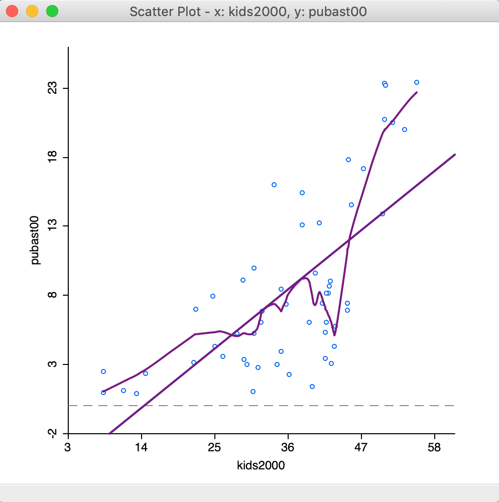
Figure 24: Default LOWESS smoother

In our example, there is considerable evidence of a nonlinear relationship between the two variables. An alternative interpretation is to see this as an indication of a structural break, where in one subset of the data the slope is very steep, whereas in another it is fairly flat.

LOWESS parameters

The nonlinear fit is driven by a number of parameters, the most important of which is the bandwidth, i.e., the range of values on the X-axis on which the local slope estimate is based.

The smoothing parameters can be changed in the options by selecting Edit LOWESS Parameters in the Smoother option. As shown in Figure 25, a small dialog is brought up in which the Bandwidth (default setting 0.20), Iterations and Delta Factor can be adjusted.

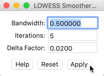
Figure 25: LOWESS bandwidth settings

The bandwidth determines the smoothness of the curve and is given as a fraction of the total range in X values. In other words, the default bandwidth of 0.20 implies that for each local fit (centered on a value for X), about one fifth of the scatter points are taken into account. The other options are technical and are best left to their default values.⁵

To obtain Figure 26, we changed the bandwidth to 0.50, which results in a much smoother curve that brings out a possible structural break in the data in a more striking fashion.

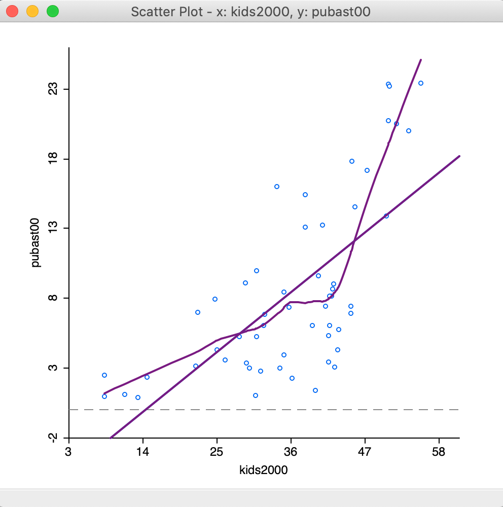
Figure 26: LOWESS smoother bandwidth 0.40

The plot seems to suggest that the linear fit is really a compromise between two slopes. There is a steep slope for observations with a value for households with children above 40 percent, suggesting a major increase in public assistance with every increase in the percentage children. With values for kids2000 below 40, the slope is much gentler and even flat in small subsets of the data.

The opposite effect is obtained when the bandwidth is made smaller. For example, with a value of 0.10, the resulting curve in Figure 27 is much more jagged and less informative.

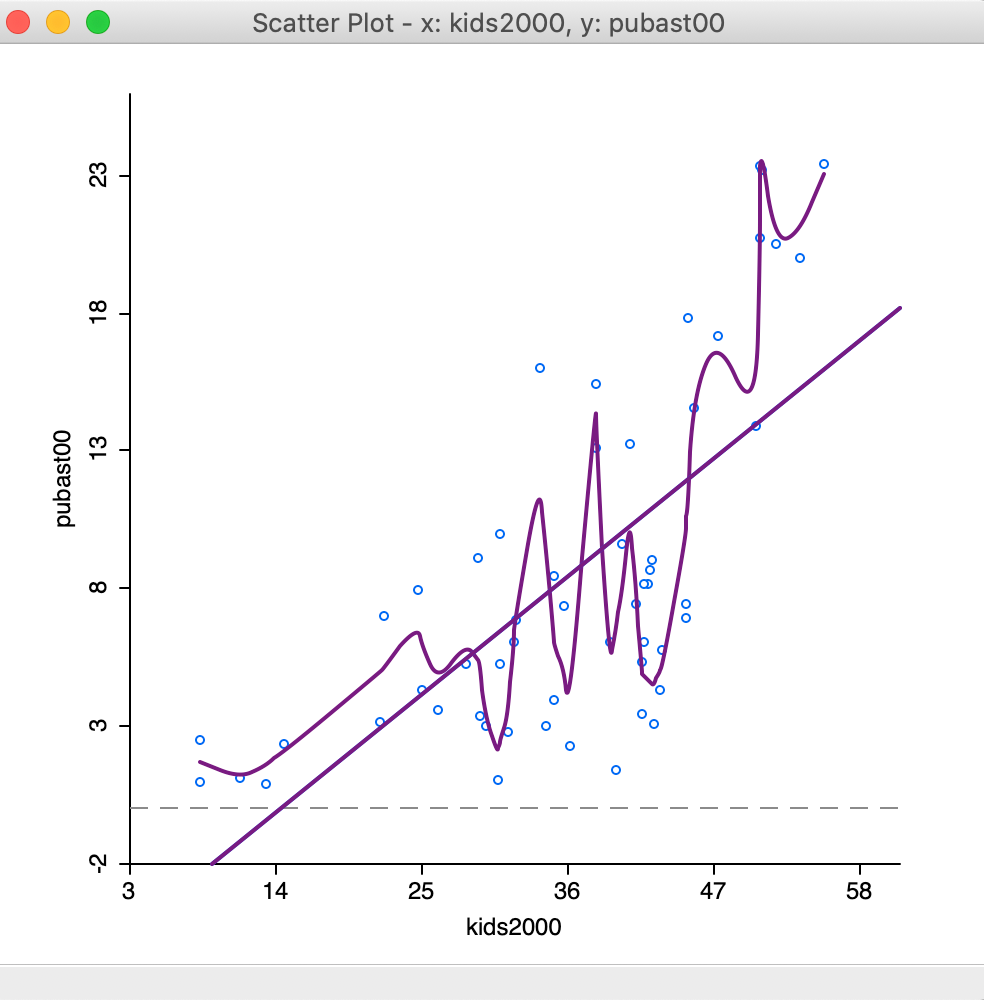
Figure 27: LOWESS smoother bandwidth 0.10

The literature contains many discussions of the notion of an optimal bandwidth, but in practice a trial and error approach is often more effective. In any case, a value for the bandwidth that follows one of these rules of thumb can be entered in the dialog. Currently, GeoDa does not compute optimal bandwidth values.

Finally, while one might expect the LOWESS fit and a linear fit to coincide with a bandwidth of 1.0, this is not the case. The LOWESS fit will be near-linear, but slightly different from a standard least squares result due to the locally weighted nature of the algorithm.

Spatial Heterogeneity

Spatial heterogeneity is one of the most important aspects of a spatial analysis of the data. In essence, its presence suggests that different distributions drive the observed sample. This is evidenced in the form of structural breaks, such as different mean or median values in different subsets of the data, or different slopes in a bivariate regression over observations in those subsets.

The spatial aspect comes from the nature of the subsets in the data, which are spatially defined. Examples are the difference between center and periphery, east and west, north and south, etc. In GeoDa, the selection tool applied to a map allows us to assess the degree of heterogeneity in different spatial subsets of the data.

We have already seen in the mapping Chapter how a selection in any of the views results in the same observation to immediately be selected in all other views through linking. Brushing is a dynamic extension of this process (for some early exposition and discussion of these ideas pertaining to so-called dynamic graphics, see, e.g., the classic references of Stuetzle 1987; Becker and Cleveland 1987; Becker, Cleveland, and Wilks 1987; Monmonier 1989; as well as in the outline of legacy GeoDa functionality in Anselin, Syabri, and Kho 2006).

Here, we will cover two particular implementations that are of interest in the context of spatial heterogeneity, one focused on differences in the mean, the other on differences in the regression slope.

Averages Chart

The Averages Chart is an implementation of a simple test on the difference in means between selected and unselected observations. Its most meaningful use is in the context of observations at different points in time, but it is equally applicable in a cross-sectional setting, illustrated here.

The core functionality of this chart is to illustrate and quantify the difference between the mean of a variable for selected observations and unselected observations (the complement). In GeoDa, this is not implemented as a traditional t-test, but rather as an F-statistic for a regression that includes an indicator variable for the selection (i.e., value = 1 for selected, and zero otherwise). The F-statistic on the significance of the joint slopes in that regression is equivalent to a t-test on the coefficient of the indicator variable, since there is only one slope.⁶

The functionality is invoked from the menu as Explore > Averages Chart, or from the toolbar, by selecting the second icon from the right, as in Figure 28.

Figure 28: Averages Chart toolbar icon

The averages chart interface, shown in Figure 29, requires that a variable be specified, as well as a selection of observations. The starting value shows the first variable in the data table, which is usually not informative. In the example in Figure 29, we have selected rent2008, as shown next to Variable in the upper left corner of the dialog. Since there is currently no selection, the Group shown as Selected has 0 observations, and a Mean of 0.00. In contrast, the Unselected consists of all 55 observations and its mean is the overall average for the rent values. In the graph on the right, the selected mean is given in red, and the unselected in blue. As it stands, this figure is not very useful, since we need to create a selection.

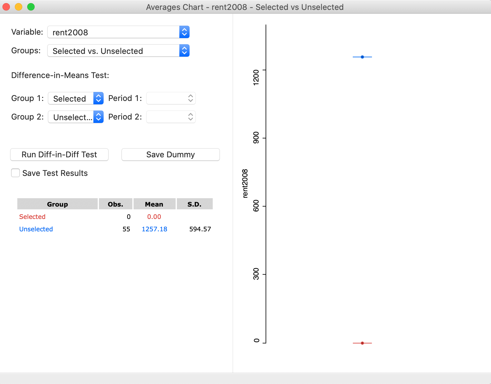
Figure 29: Averages Chart with variable selected

We select all the observations for Manhattan. This is straightforward by means of the Selection Tool in the data table. As it turns out, all the sub-boroughs in Manhattan have a value for bor_subb between 301 and 310, which provides an easy way to select them. With that selection in place, the values in the averages chart are immediately adjusted, as shown in Figure 30. In the updated dialog, the Selected consist of 10 observations, with a mean rent of 2062.5, which contrasts with the mean for the Unselected of 1078.22. In the graph on the right, again, the selected mean is shown as the red bar and the unselected one as the blue bar. In the middle, as a black bar, is the overall mean (for all the observations).

At this point, the result for an F-test on the slope of the dummy variable regression is available as well. The statistic has a value of 37.63, for 1, 53 degrees of freedom, which yields a highly significant p-value of 0.000.⁷ Note that this statistic does not account for heteroskedasticity or the potential presence of spatial autocorrelation, which is beyond our current scope.

The averages chart provides an easy method to test for the difference in means between two subsets of the data. This becomes a test for spatial heterogeneity when the selected subsets are spatial in nature. In our current example, we obtained a spatial selection by coincidence (by selecting on the id-values for Manhattan). Next, we consider a true spatial selection.

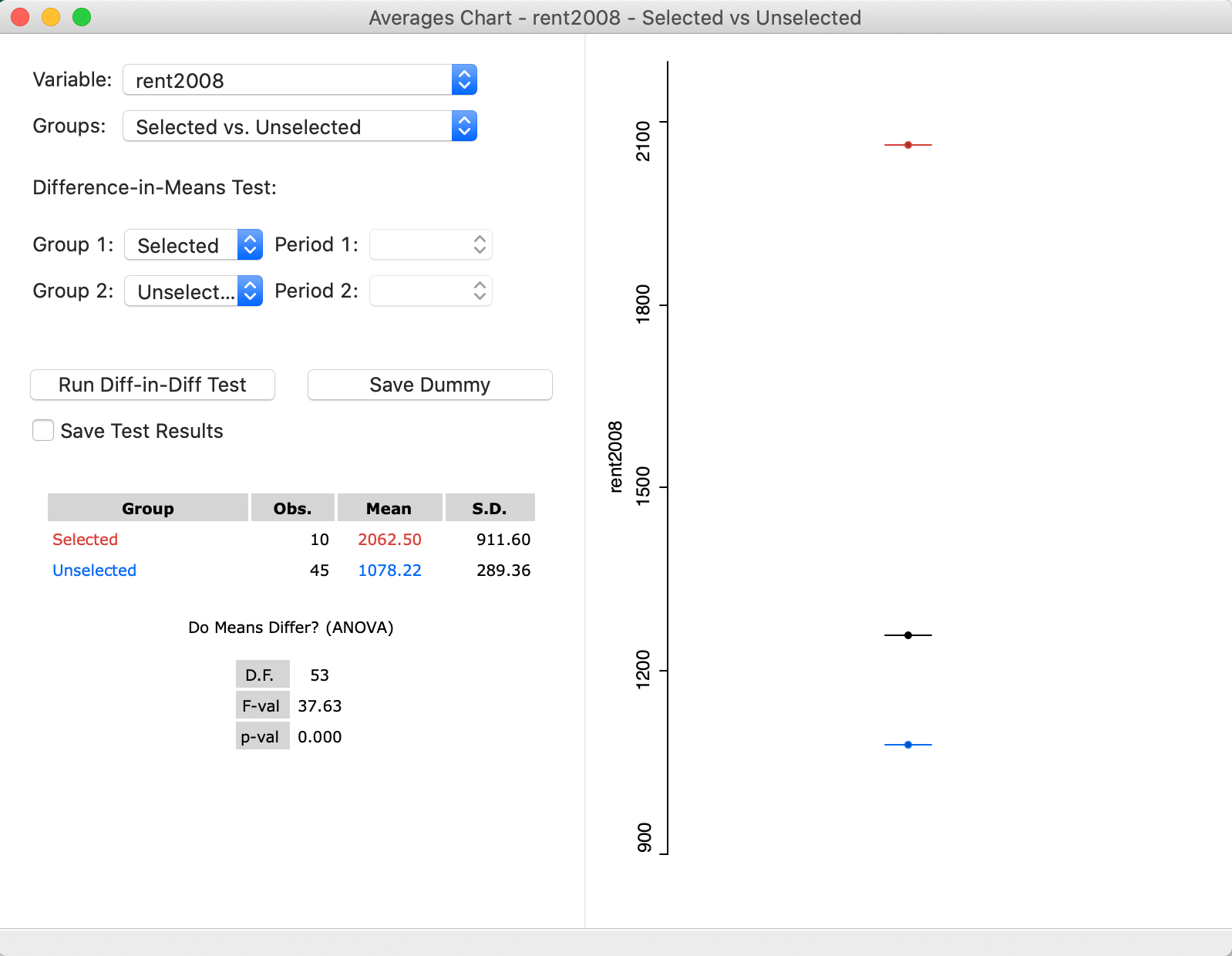
Figure 30: Averages Chart for rent2008 with Manhattan-The Bronx

Map brushing and the Averages Chart

The real power to assess spatial heterogeneity in the means comes from employing the brush in a map. As the dynamic version of linking, the brush (e.g., a rectangle) is moved over the map and continuously updates the selection of observations. As soon as the brush stops moving, the test on the difference in means is updated in the averages chart, allowing us to assess for which subregions the differences are the greatest.

For example, in Figure 31, we start with a selection in the lower right of the map, covering parts of Queens and Brooklyn. The respective average rents are 1150 for the 21 selected observations (red bar, below the overall mean), and 1323.38 for the 34 unselected (blue). The difference between the two is insufficient to yield a significant F-test. With a statistic of 1.11, the associated p-value is 0.298, insufficient to reject the null hypothesis of equality of the means.

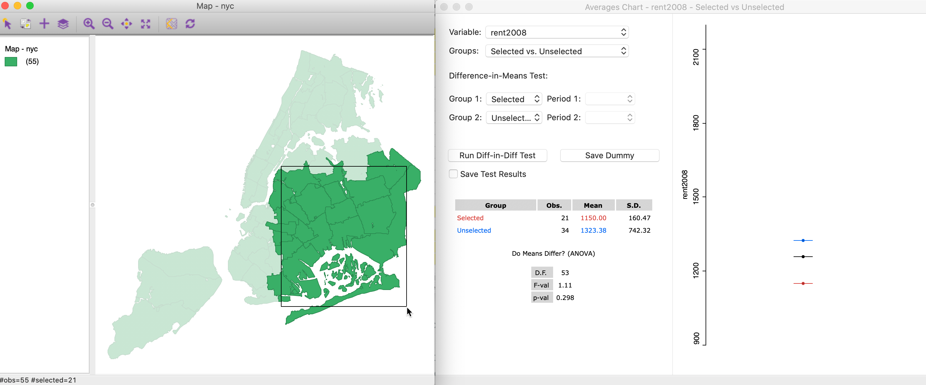
Figure 31: Brushing with the Averages Chart (1)

As we move the brush west and north, the situation changes. Now, the mean for the 22 selected observations of 1517.05 (red bar) is above the overall mean, and compares for an average of 1083.94 for the 33 unselected observations. The F statistic of 7.90 obtains a p-value of 0.007, clearly rejecting the null hypothesis and indicating spatial heterogeneity in the means.

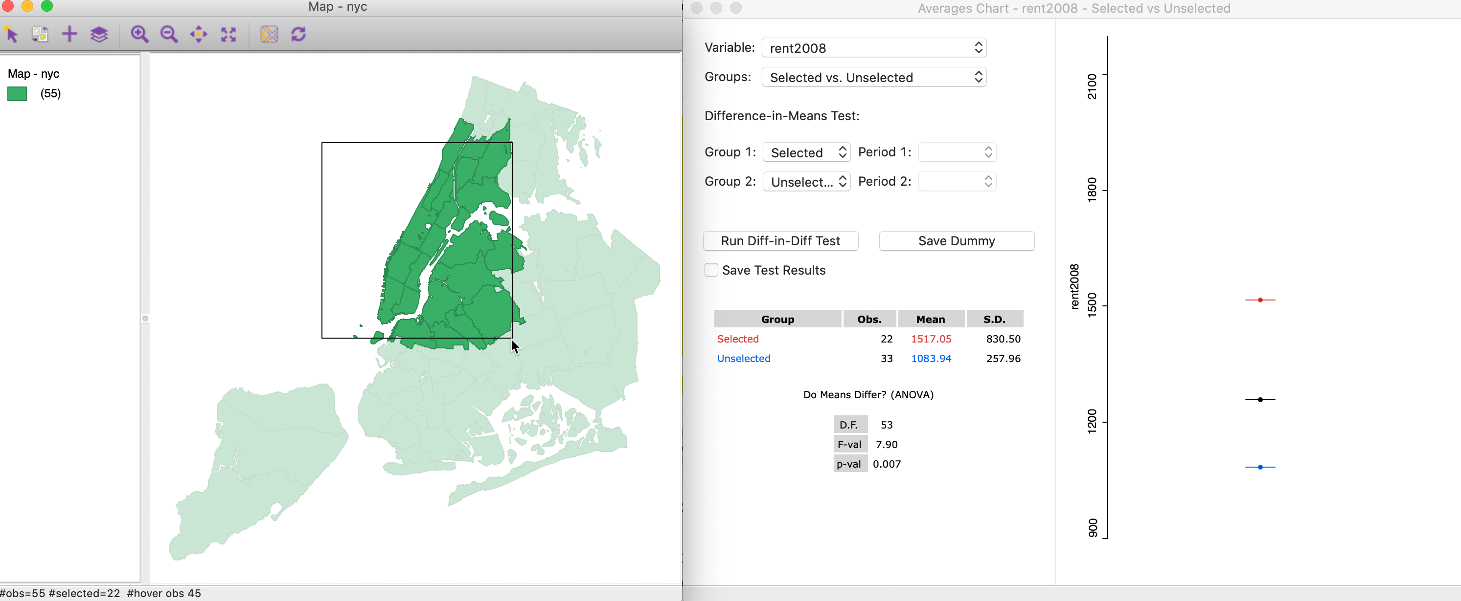
Figure 32: Brushing with the Averages Chart (2)

Brushing the Scatter Plot

The concept of brushing was initially suggested in the context of a scatter plot (Stuetzle 1987), and extended to the map context by Monmonier (1989). The architecture linking all open windows simultaneously is fundamental to the design of GeoDa (Anselin, Syabri, and Kho 2006).

We illustrate brushing of the scatter plot with the example of kids2000 and pubast00, intitialized in Figures 19 and 20. We initiate the brushing process by setting up a selection shape in the scatter plot. The default is a rectangular shape, but we have seen earlier how that can be changed to a circle or a line. In our example, we keep the default.

We click at a given location in the scatter plot and draw the pointer into a rectangular shape, as shown in Figure 33. Note how the pointer is attached to a corner of the rectangle. At this point, the shape can be moved around in the view, dynamically changing the selection.

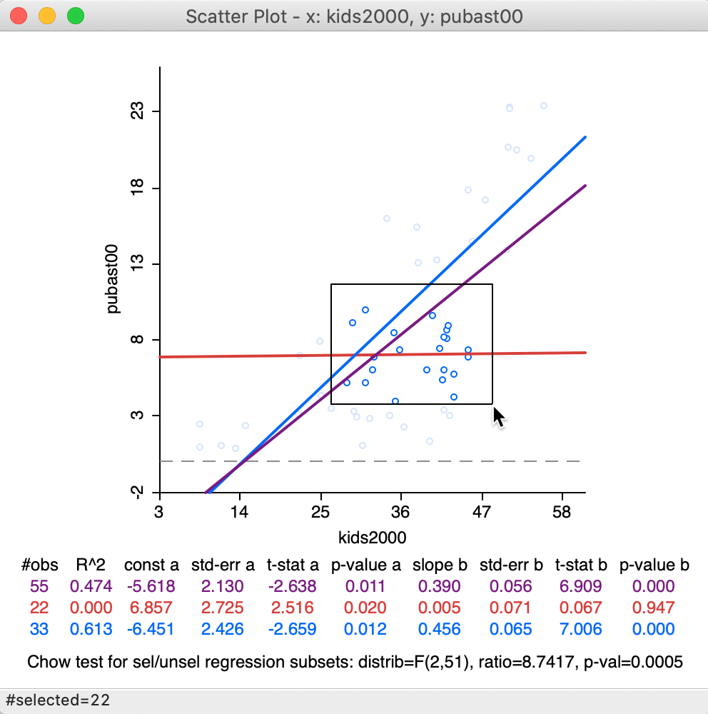
Figure 33: Brushing the scatter plot – 1

In our example, we have selected 22 observations. The purple line represents the original linear fit, the red line is the fit for the 22 selected observations, and the blue line is the fit for the other 33 observations. Below the three lines with the slope coefficients and fit statistics, the results are listed of a Chow test on structural stability are listed (Chow 1960).⁸ Clearly, in contrast to the overall purple and the blue line, there is no relationship at all for the selected observations in question, as evidenced by the horizontal red line. The Chow test confirms this by strongly rejecting (p < 0.0005) the null hypothesis of equal coefficients (between the slopes of the blue and the red lines).

Because of the linking, the 22 selected observations are also highlighted in all the other views. Such views could pertain to the same or to different variables, allowing us to investigate potential interaction effects.

With the Regimes Regression option turned on, the three linear fits change instantaneously as different observations are selected. Of course, the fits themselves are only meaningful when sufficient observations are part of the selection. For example, we can move the selection rectangle up and to the right, as in Figure 34, which yields a new selection of 11 observations, with associated regression lines. This time, there is insufficient evidence to reject the null hypothesis (Chow test with p = 0.9513).

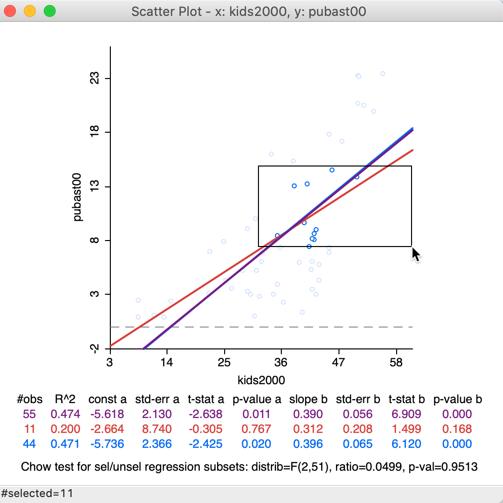
Figure 34: Brushing the scatter plot – 2

Again, the matching selected locations are shown in all the other current views.

Map brushing and scatter plot

Similar to what we saw for the averages chart, a powerful assessment of potential spatial heterogeneity in a bivariate linear regression is based on brushing a map, linked to a scatter plot.

As before, we start by making a selecting in a map. For example, in Figure 35, 17 observations are selected. This selection is reflected in a new set of slopes in the scatter plot. In this case, the difference between the red (selected) and blue (unselected) slopes is insufficient to lead to a rejection of the null hypothesis by means of the Chow test (a p-value of 0.1693).

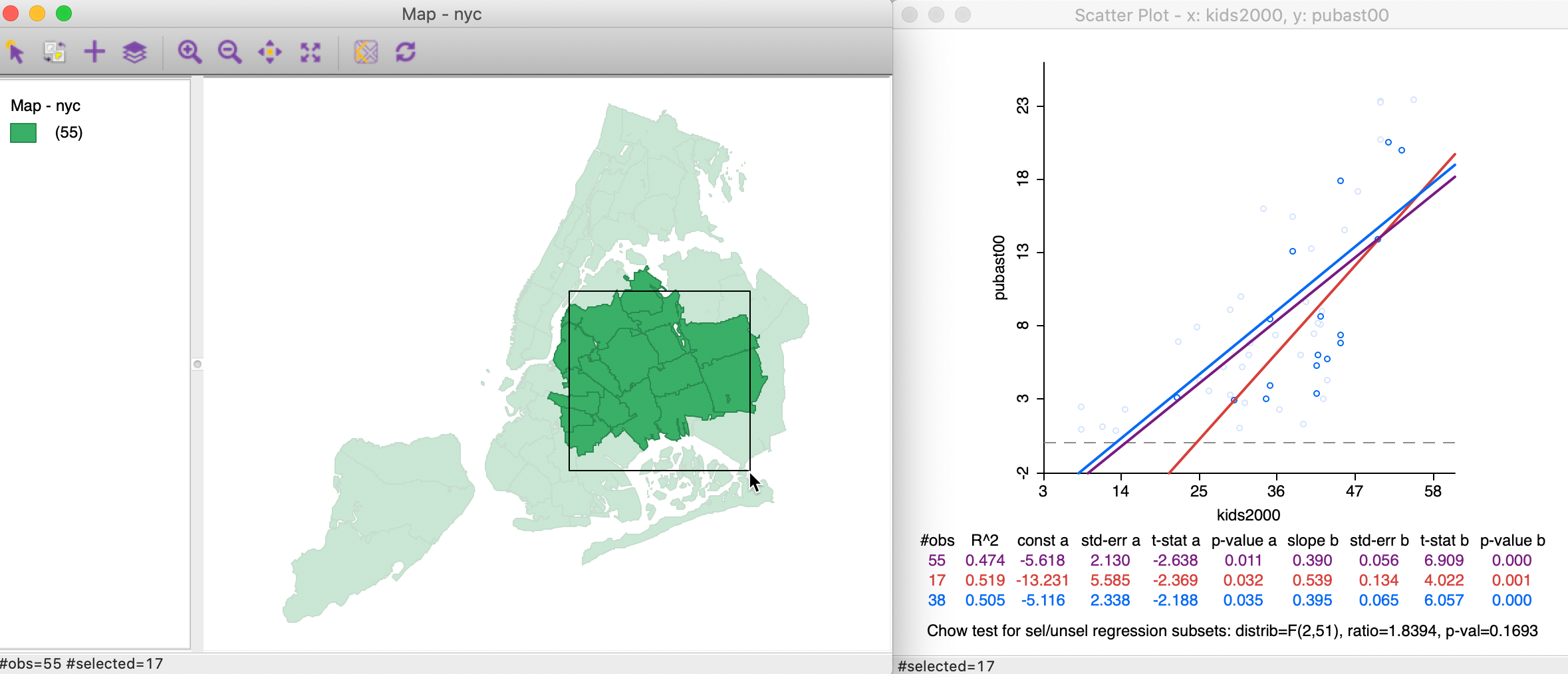
Figure 35: Brushing a map linked to a scatter plot – 1

As we brush across the map, we can assess the degree to which the linear relationship is stable. Any systematically changing slopes between clearly defined sub-regions of the observations would suggest the presence of spatial heterogeneity.

For example, moving the selection rectangle to the north and west, as in Figure 36, makes the evidence for structural change much stronger, as evidenced by the Chow test with p < 0.0005.

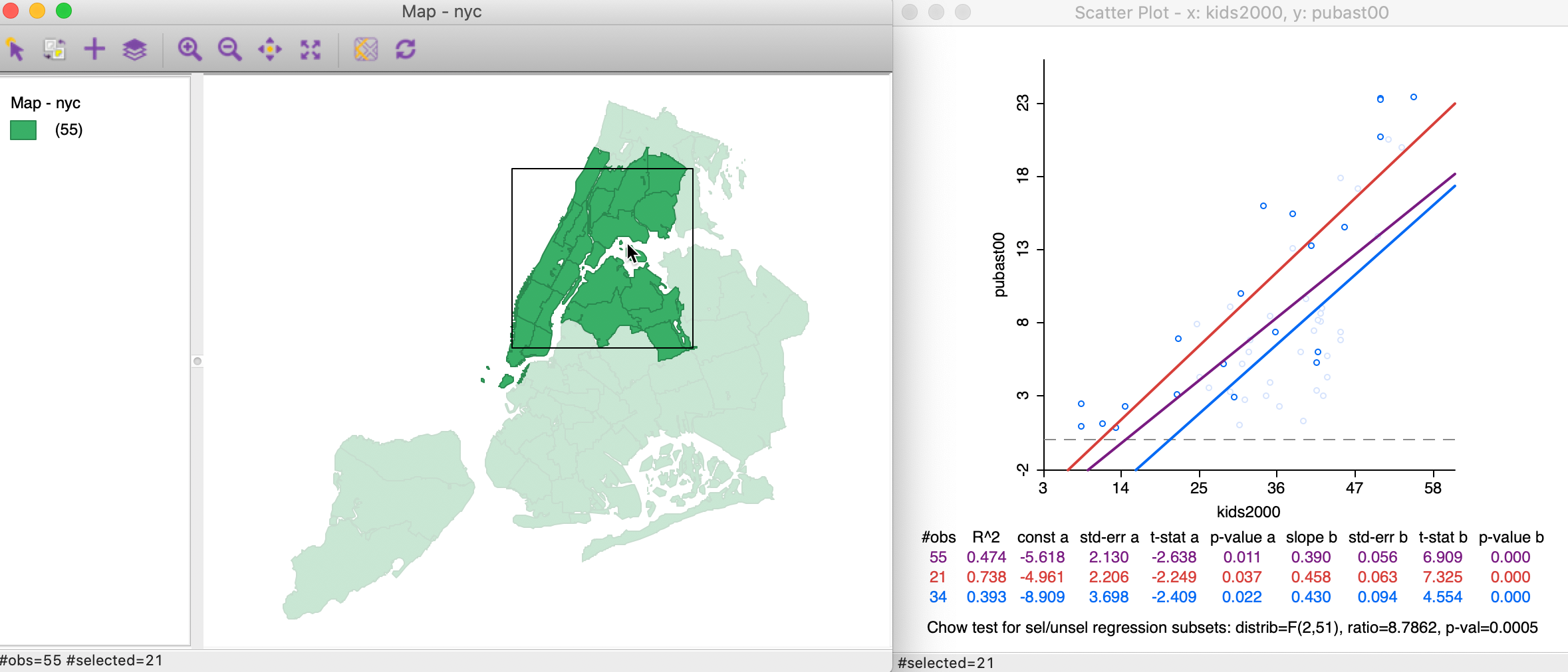
Figure 36: Brushing the map – 2

As we identify subregions in the data with a different slope (structure) from the rest, we can assess this more formally through regression analysis (e.g., analysis of variance). This is facilitated by Saving the selection in the form of an indicator variable (with 1 for the selected observations).

The new variable can then be incorporated in a regression specification, potentially interacting with other explanatory variables, to more formally address spatial regimes.⁹

References

Anselin, Luc, and Sergio J. Rey. 2014. Modern Spatial Econometrics in Practice, a Guide to Geoda, Geodaspace and Pysal. Chicago, IL: GeoDa Press.

Anselin, Luc, Ibnu Syabri, and Youngihn Kho. 2006. “GeoDa, an Introduction to Spatial Data Analysis.” Geographical Analysis 38: 5–22.

Becker, Richard A., and W. S. Cleveland. 1987. “Brushing Scatterplots.” Technometrics 29: 127–42.

Becker, Richard A., W. S. Cleveland, and A. R. Wilks. 1987. “Dynamic Graphics for Data Analysis.” Statistical Science 2: 355–95.

Chow, G. 1960. “Tests of Equality Between Sets of Coefficients in Two Linear Regressions.” Econometrica 28: 591–605.

Cleveland, William S. 1979. “Robust Locally Weighted Regression and Smoothing Scatterplots.” Journal of the American Statistical Association 74: 829–36.

Loader, Catherine. 1999. Local Regression and Likelihood. Heidelberg: Springer-Verlag.

———. 2004. “Smoothing: Local Regression Techniques.” In Handbook of Computational Statistics: Concepts and Methods, edited by James E. Gentle, Wolfgang Härdle, and Yuichi Mori, 539–63. Berlin: Springer-Verlag.

Monmonier, Mark. 1989. “Geographic Brushing: Enhancing Exploratory Analysis of the Scatterplot Matrix.” Geographical Analysis 21: 81–84.

Stuetzle, W. 1987. “Plot Windows.” Journal of the American Statistical Association 82: 466–75.

---

1. University of Chicago, Center for Spatial Data Science – anselin@uchicago.edu↩︎

2. Consult the mapping chapter if you are unsure of how to accomplish this.↩︎

3. In the GeoDa Preference Setup, under System, the transparency of the unhighlighted objects in a selection operation can be adjusted. The default is 0.80, which means only about 20% of the regular color is shown.↩︎

4. Note that the fences are drawn even when they fall outside the actual range of the observations. This will be the case whenever the value of the third quartile + 1.5xIQR is larger than the maximum, (as in in Figure 16), or when the value of the first quartile - 1.5xIQR is smaller than the minimum.↩︎

5. The LOWESS algorithm is complex and uses a weighted local polynomial fit. The Iterations setting determines how many times the fit is adjusted by refining the weights. A smaller value for this option will speed up computation, but result in a less robust fit. The Delta Factor drops points from the calculation of the local fit if they are too close (within Delta) to speed up the computations. Technical details are covered in Cleveland (1979).↩︎

6. The F-statistic is basically a test on whether there is a significant gain in explanation in the regression beyond the overall mean (i.e., the constant term). Formally, the statistic uses the sum of squared residuals in the regression RSS and the sum of squared deviations from the mean for the dependent variable RSY. The statistic follows as: \[F = \frac{RSS - RSY}{k - 1} / \frac{RSY}{n - k},\] with \(k\) as the number of explanatory variables. In our simple dummy variable regression, \(k = 2\), so that the degrees of freedom for the F-statistic are \(1, n-2\). See also Anselin and Rey (2014), pp. 98-99.↩︎

7. Since the first degree of freedom of the F-test in this case is always 1, it is not reported. Therefore, the entry for D.F. is 53, which corresponds to n - k = 55 - 2.↩︎

8. The Chow test is based on a comparison of the fit in the overall regression to the combination of the fits of the separate regressions, while taking into account the number of regressors (k). In our simple example, there is only the intercept and the slope, so k = 2. We compute the residual sum of squares for the full regression (\(\mbox{RSS}\)) and for the two subsets, say \(\mbox{RSS}_1\) and \(\mbox{RSS}_2\). Then, the Chow test follows as: \[C = \frac{(\mbox{RSS} - (\mbox{RSS}_1 + \mbox{RSS}_2))/k}{(\mbox{RSS}_1 + \mbox{RSS}_2)/(n - 2k)},\] distributed as an F statistic with \(k\) and \(n - 2k\) degrees of freedom. Alternatively, the statistic can also be expressed as having a chi-squared distribution, which is more appropriate when multiple breaks and several coefficients are considered. Technical details are given in Anselin and Rey (2014), pp. 287-289.↩︎

9. the treatment of spatial regimes is beyond our current scope. For a detailed technical discussion, see Anselin and Rey (2014), part IV.↩︎

GeoDa is maintained by lixun910. This page was generated by GitHub Pages using the Cayman theme by Jason Long.