Maps for Rates or Proportions
Luc Anselin1
08/03/2018 (revised and updated)
Introduction
In this chapter, we will explore some important concepts that are relevant when mapping rates or proportions. Such data are characterized by an intrinsic variance instability, in that the precision of the rate as an estimate for underlying risk is inversely proportional to the population at risk. Specifically, this implies that rates estimated from small populations (e.g., small rural counties) may have a large standard error. Furthermore, such rate estimates may potentially erroneously suggest the presence of outliers.
In what follows, we will cover two basic methods to map rates. We will also consider the most commonly used rate smoothing technique, based on the Empirical Bayes approach. Spatially explicit smoothing techniques will be treated after we cover distance-based spatial weights.
Objectives
-
Obtain a coordinate reference system
-
Create thematic maps for rates
-
Assess extreme rate values by means of an excess risk map
-
Understand the principle behind shrinkage estimation or smoothing rates
-
Apply the Empirical Bayes smoothing principle to maps for rates
-
Compute crude rates and smoothed rates in the table
GeoDa functions covered
- Map > Rates-Calculated Map
- Raw Rate
- Excess Risk
- Empirical Bayes
- saving calculated rates to the table
- Table > Calculator > Rates
- Raw Rate
- Excess Risk
- Empirical Bayes
Getting started
In this chapter, we will use a sample data set with lung cancer data for the 88 counties of the state of Ohio. This is a commonly used example in many texts that cover disease mapping and spatial statistics.2 The data set is also included as one of the Center for Spatial Data Science example data sets and can be downloaded from the Ohio Lung Cancer Mortality page.
After the zipped file is downloaded, we select the three files in the ohiolung folder that are associated with the ESRI shape file format: ohlung.shp, ohlung.shx, and ohlung.dbf. Note that there is no projection file available (no ohlung.prj file). However, the metadata file ohiolung_metadata.html refers to the county boundary file as being in the UTM Zone 17 projection.
Digression - finding the right projection for a map
To find the correct projection metadata, we resort to the spatialreference.org site, which contains thousands of spatial references in a variety of commonly used formats. Specifically, after a few steps, we reach the page shown in Figure 1.3 The UTM Zone 17 has a EPSG code of 32617 (EPSG stands for European Petroleum Survey Group and is a commonly used system to classify coordinate reference systems and projections).
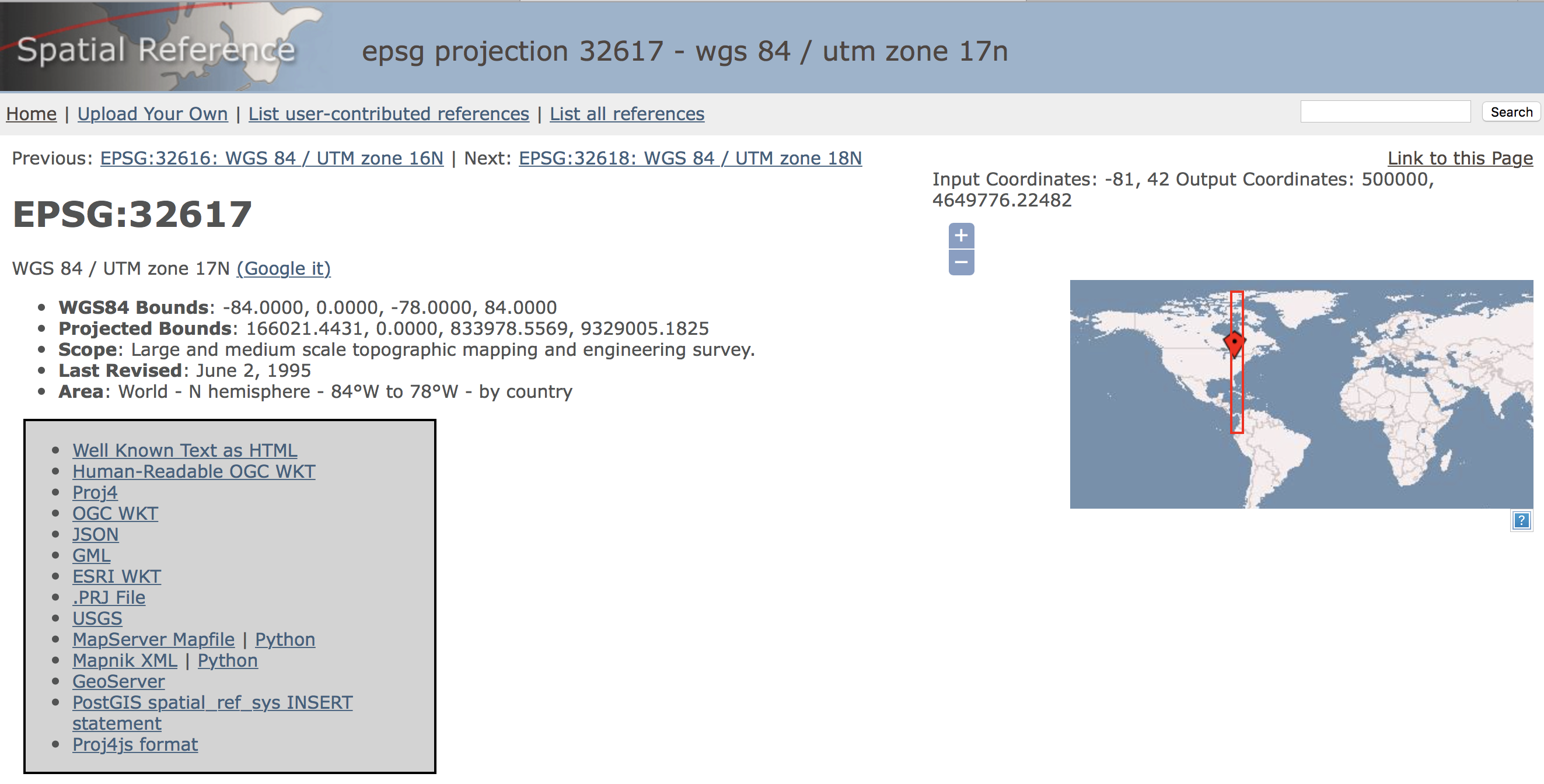
Figure 1: UTM Zone 17 projection
We can now select the .PRJ File link from the various options to download the file with the correct projection information. To match it up with our other files, we rename the file as ohlung.prj. We now have all the pieces to get started.
Further preliminaries
We fire up GeoDa, click on the Open icon and drop the ohlung.shp file in the Drop files here box of the Connect to Data Source dialog. The green themeless map with the outlines of the 88 Ohio counties appears in a map window, as in Figure 2.
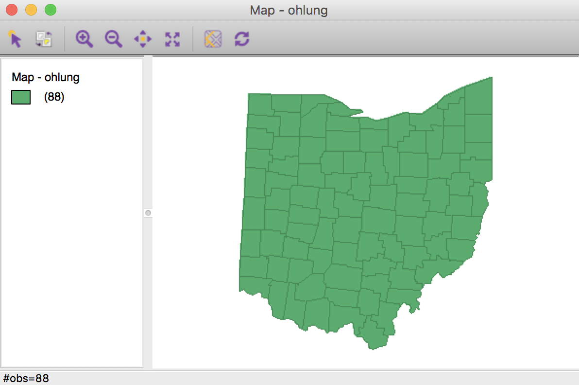
Figure 2: Ohio counties themeless map
Since we have projection information, we can add a base layer to provide some context. For example, in Figure 3, we have selected Nokia Day from the options in the Base Map icon.
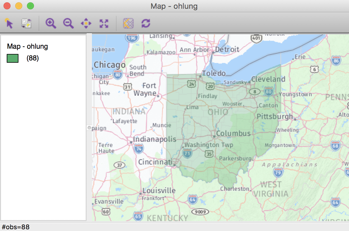
Figure 3: Ohio counties with base layer
Choropleth Map for Rates
Spatially extensive and spatially intensive variables
We start our discussion of rate maps by illustrating something we should not be doing. This pertains to the important difference between a spatially extensive and a spatially intensive variable. In many applications that use public health data, we typically have access to a count of events, such as the number of cancer cases (a spatially extensive variable), as well as to the relevant population at risk, which allows for the calculation of a rate (a spatially intensive variable).
In our example, we could consider the number (count) of lung cancer cases by county among white females in Ohio (say, in 1968). The corresponding variable in our data set is LFW68. We can create a box map (hinge 1.5) in the by now familar way, e.g., from the menu as Map > Box Map (Hinge = 1.5). To provide some context, we add a base layer using the Carto Light option. This yields the map shown in Figure 4.
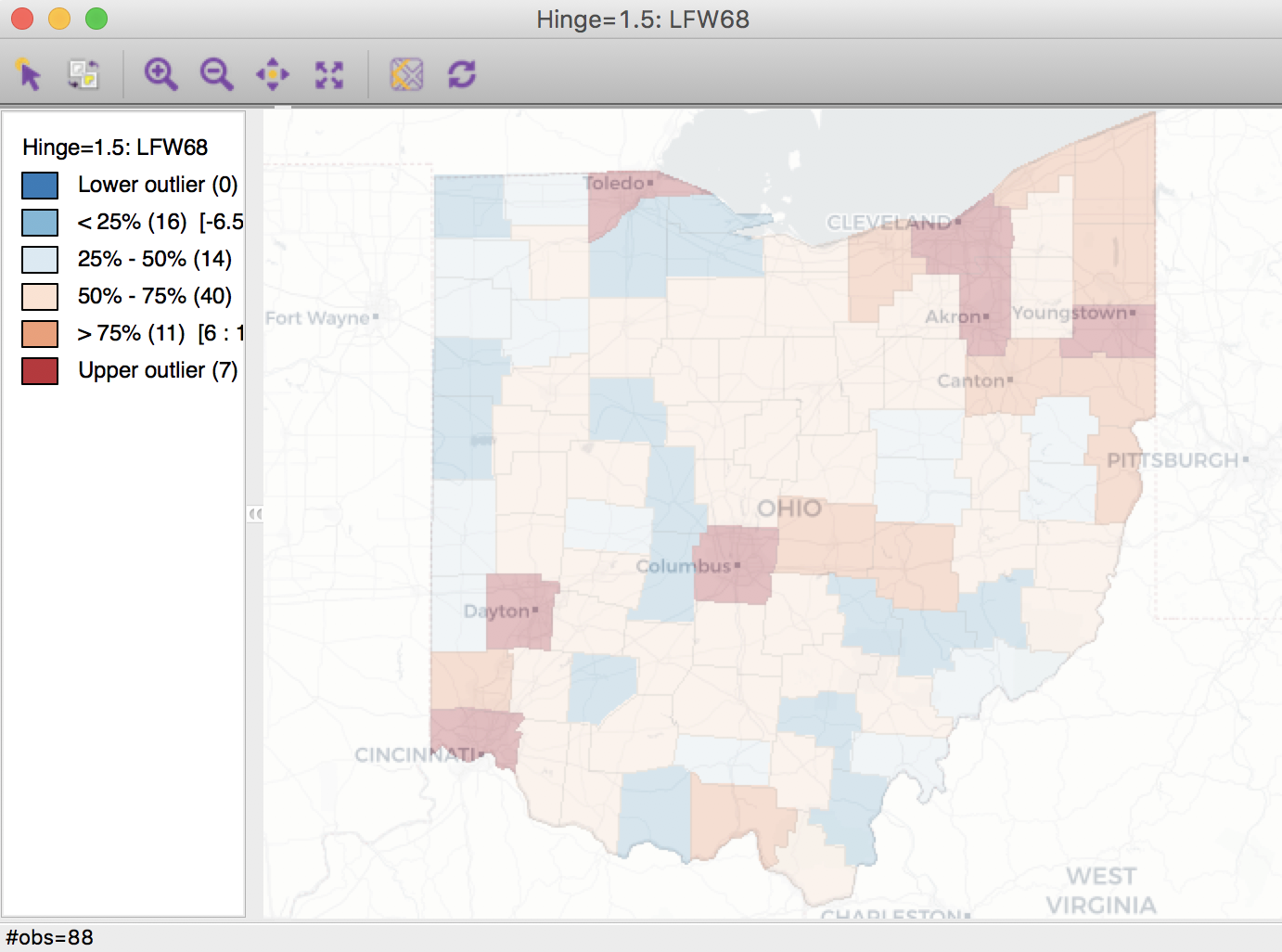
Figure 4: Spatially extensive lung cancer counts
Anyone familiar with the geography of Ohio will recognize the outliers as the counties with the largest populations, i.e., the metropolitan areas of Cincinnati, Columbus, Cleveland, etc. The labels for these cities in the base layer make this clear. This highlights a major problem with spatially extensive variables like total counts, in that they tend to vary with the size (population) of the areal units. So, everything else being the same, we would expect to have more lung cancer cases in counties with larger populations.
Instead, we opt for a spatially intensive variable, such as the ratio of the number of cases over the population. More formally, if \(O_i\) is the number of cancer cases in area \(i\), and \(P_i\) is the corresponding population at risk (in our example, the total number of white females), then the raw or crude rate or proportion follows as: \[r_i = \frac{O_i}{P_i}.\]
Variance instability
The crude rate is an estimator for the unknown underlying risk. In our example, that would be the risk of a white woman to be exposed to lung cancer. The crude rate is an unbiased estimator for the risk, which is a desirable property. However, its variance has an undesirable property, namely \[Var[r_i] = \frac{\pi_i (1 - \pi_i)}{P_i},\] where \(\pi_i\) is the underlying risk in area \(i\).4 This implies that the larger the population of an area (\(P_i\) in the denominator), the smaller the variance for the estimator, or, in other words, the greater the precision.
The flip side of this result is that for areas with sparse populations (small \(P_i\)), the estimate for the risk will be imprecise (large variance). Moreover, since the population typically varies across the areas under consideration, the precision of each rate will vary as well. This variance instability needs to somehow be reflected in the map, or corrected for, to avoid a spurious representation of the spatial distribution of the underlying risk. This is the main motivation for smoothing rates, to which we return below.
Raw rate map
The range of choropleth maps that can be constructed for rates is available from the main map menu as Map > Rates-Calculated Map. This provides five different options to calculate the rates directly from the respective counts (numerator) and populations at risk (denominator), as shown in Figure 5. For now, we will focus on the Raw Rate option.
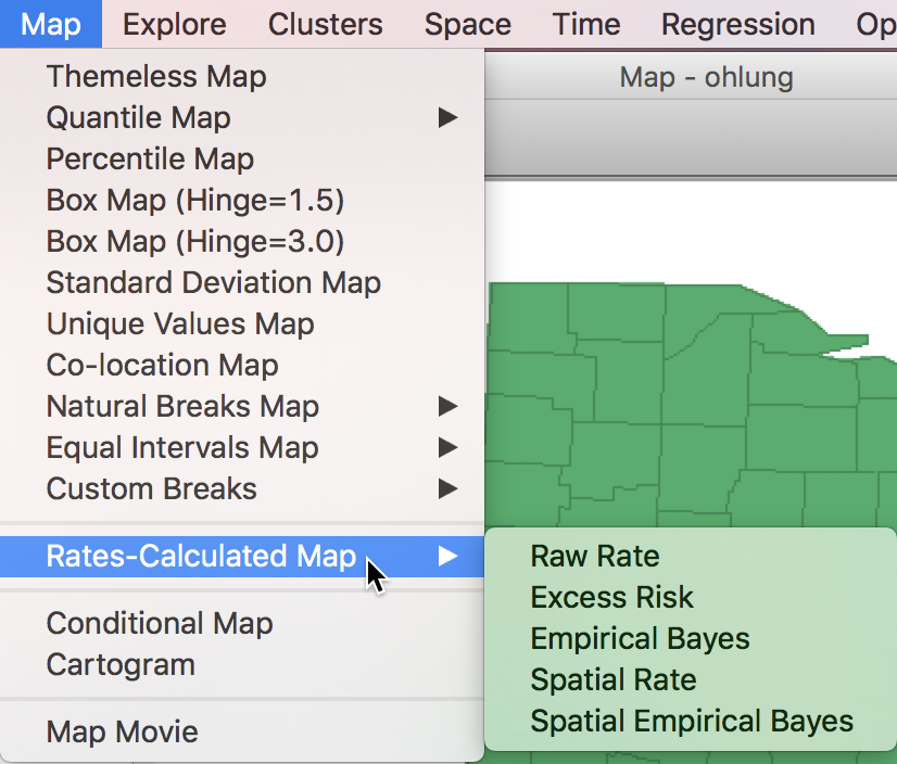
Figure 5: Rate map from main Map menu
The same five options can also be accessed from any open map through the map options menu (right click on the map) as Rates, as in Figure 6.
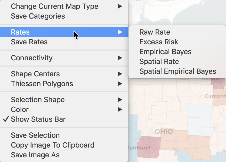
Figure 6: Rate map from Map options menu
First, we consider the Raw Rate or crude rate (proportion), the simple ratio of the events (number of lung cancer cases) over the population at risk (the county population).5 In the variable dialog shown in Figure 7, we select LFW68 as the Event Variable (i.e., the numerator) and POPFW68 as the Base Variable (i.e., the denominator). In the Map Themes drop down list, we choose Box Map (Hinge=1.5) (if we don’t specify the type of map explicitly, the default will be a quantile map with 4 categories).
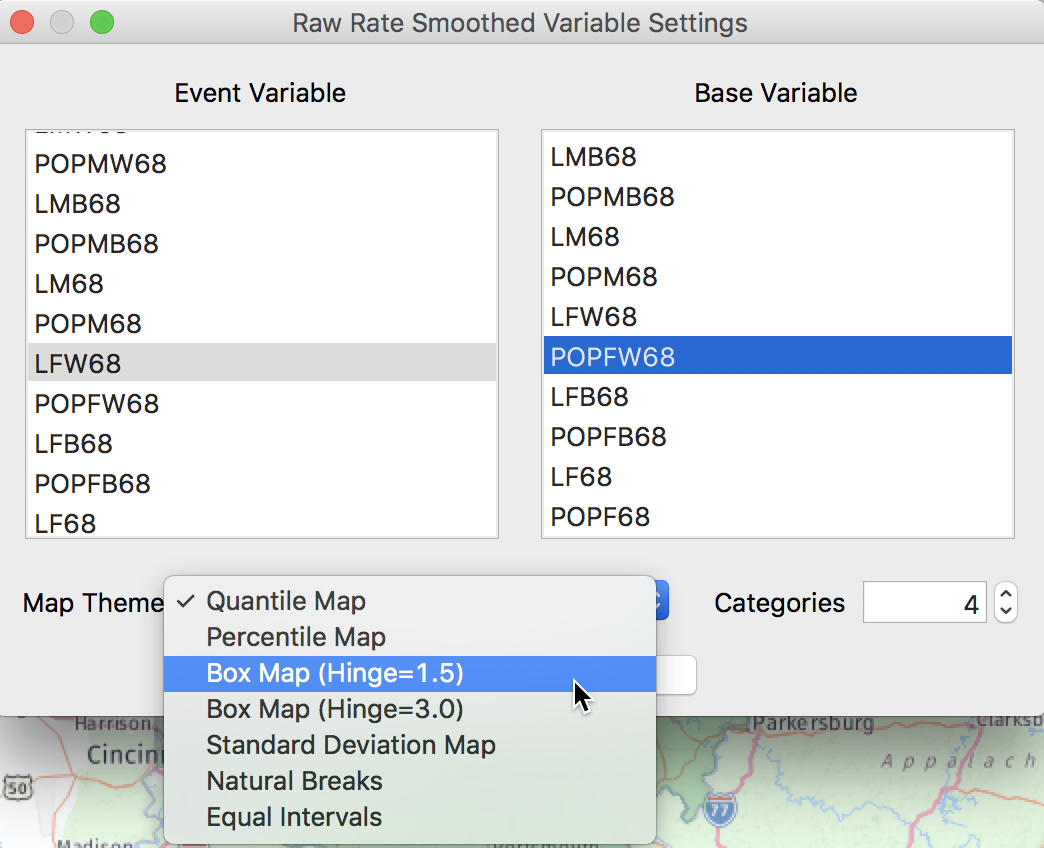
Figure 7: Lung cancer rate variables
The associated box map is shown in Figure 8.
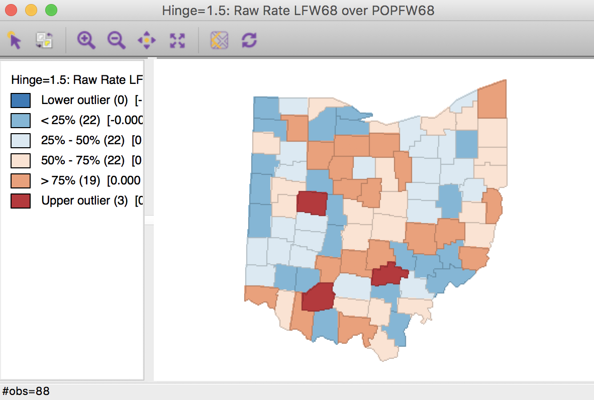
Figure 8: Lung cancer rate box map
We immediately notice that the counties identified as upper outliers in Figure 8 are very different from what the map for the counts suggested in Figure 4.
We can address this even more precisely by selecting the outliers in the count map (click on the square in the legend next to Upper outlier), and identify the corresponding counties in the rate map through linking. In Figure 9, they are shown in the actual shade, whereas the non-selected counties are shown in a lower transparency. None of the original count outliers remain as extreme values in the rate map. In fact, some counties are in the lower quartiles (blue color) for the rates.
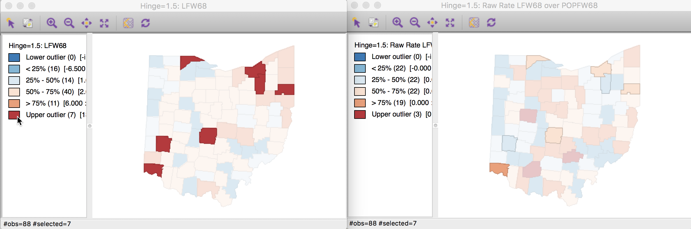
Figure 9: Count outliers in rate map
This highlights the problem with using spatially extensive variables to assess the spatial pattern of events. The only meaningful analysis is when the population at risk (the denominator) is also taken into account through a rate measure.
Saving the rates to the table
Even though we have a map for the lung cancer mortality rates, as such, the rates themselves are not available for any other analyses. However, this can be easily remedied. A right click in the map will bring up the familiar map options menu (for example, see Figure 6), from which Save Rates can be selected to create the rate variable. This brings up a dialog to specify a name for the rate variable if one wants something different than the default. For example, we can use RLFW68, as shown in Figure 10.
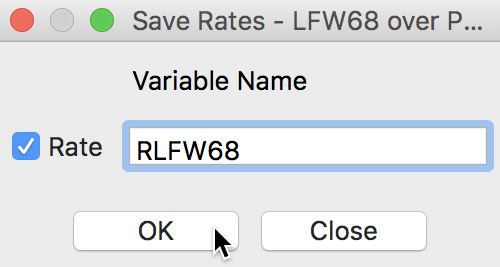
Figure 10: Rate variable name selection
After clicking on OK, the new variable is added to the table. We can verify this by bringing the table to the foreground (click on the Table icon in the toolbar). The new variable has been added as the last field in the table, as in Figure 11.
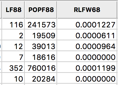
Figure 11: Rate field added to table
As usual, in order to make this new variable a permanent part of the data set, we need to Save the current data set, or Save As a new data set.
Computing rates in the table
Rates can also be computed through the Calculator functionality for the table (Table > Calculator). In the calculator dialog shown in Figure 12, we select the Rates tab, which has the same five rate calculation options as before available under the Method drop down list.
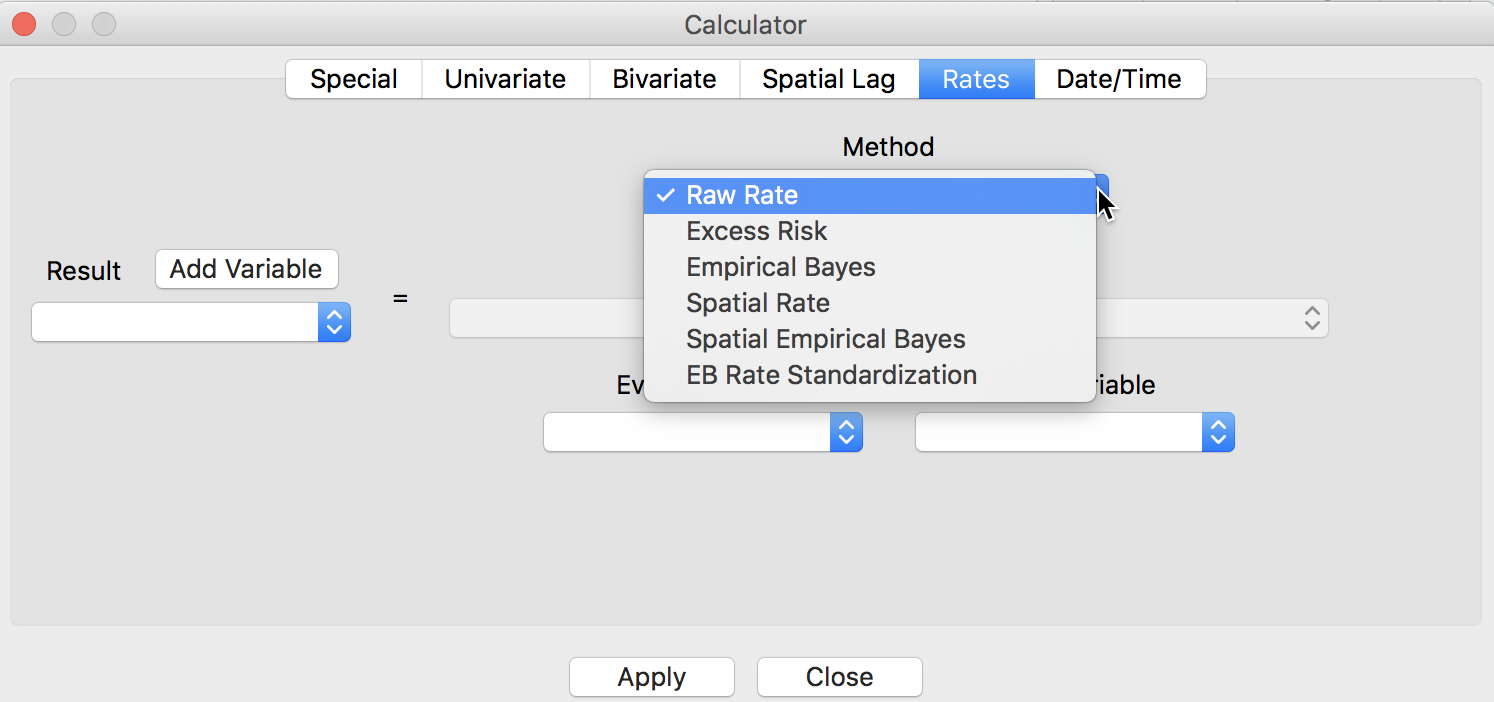
Figure 12: Rate computation in table calculator
To calculate the rates, we operate in the customary fashion, by first adding a variable (say, LRATE)6 and then performing the computation. After selecting Raw Rate as the Method, we pick LFW68 as the Event Variable and POPFW68 as the Base Variable in the dialog, as illustrated in Figure 13.
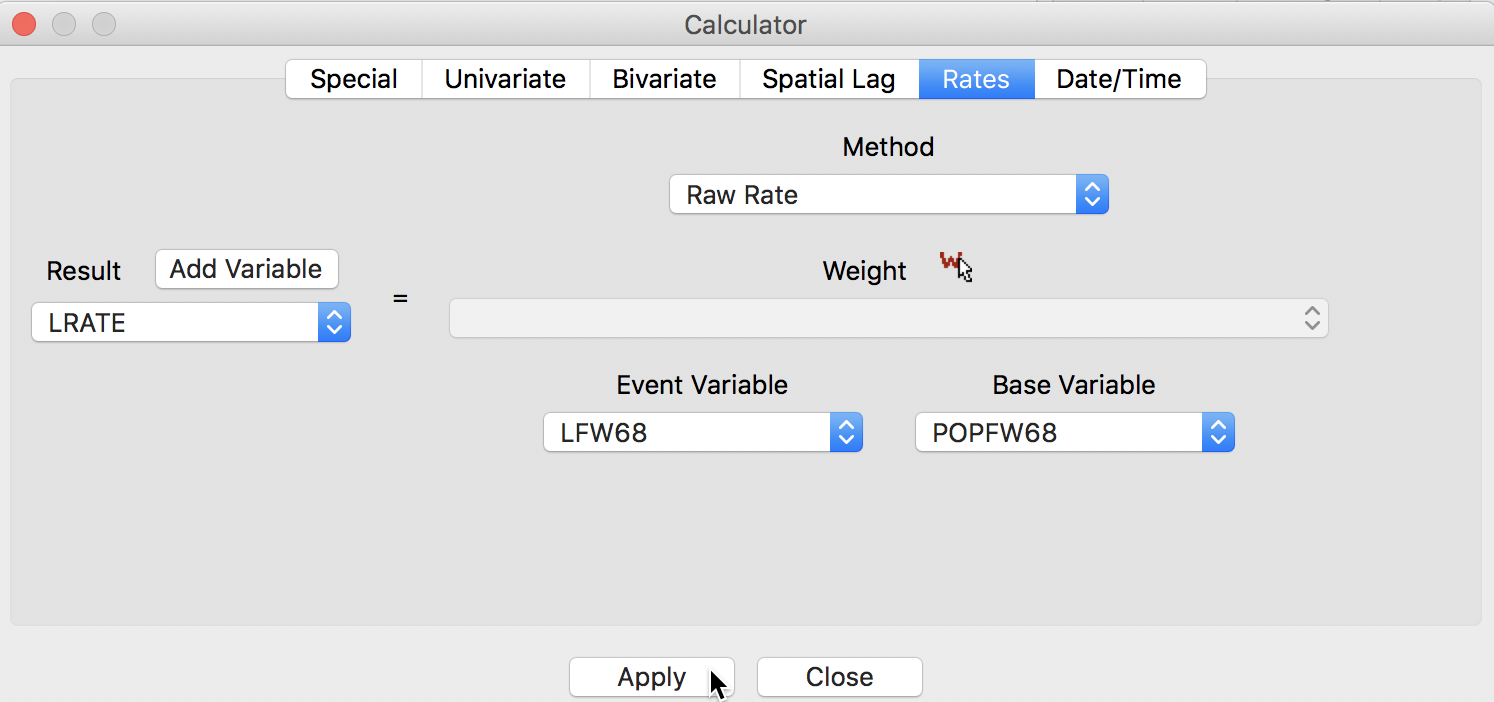
Figure 13: Rate variables in table calculator
After clicking Apply, the new variable is added to the table, as in Figure 14.
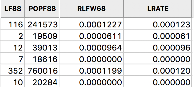
Figure 14: Rate field added to table
As before, in order to make this permanent, we neede to Save or Save As.
Excess Risk
Relative risk
A commonly used notion in demography and public health analysis is the concept of a standardized mortality rate (SMR), sometimes also referred to as relative risk or excess risk. The idea is to compare the observed mortality rate to a national (or regional) standard. More specifically, the observed number of events is compared to the number of events that would be expected had a reference risk been applied.
In most applications, the reference risk is estimated from the aggregate of all the observations under consideration. For example, if we considered all the counties in Ohio, the reference rate would be the sum of all the events over the sum of all the populations at risk. Note that this average is not the average of the county rates. Instead, it is calculated as the ratio of the total sum of all events over the total sum of all populations at risk (e.g., in our example, all the white female deaths in the state over the state white female population). Formally, this is expressed as: \[\tilde{\pi} = \frac{\sum_{i=1}^{i=n} O_i}{\sum_{i=1}^{i=n} P_i},\] which yields the expected number of events for each area \(i\) as: \[E_i = \tilde{\pi} \times P_i.\] The relative risk then follows as the ratio of the observed number of events (e.g., cancer cases) over the expected number: \[SMR_i = \frac{O_i}{E_i}.\]
Excess risk map
We can map the standardized rates directly by means of Rates-Calculated Map > Excess Risk item in the map menu. In the dialog that follows, shown in Figure 15, we specify the same variables as before for Event Variable (LFW68) and for the Base Variable (POPFW68).
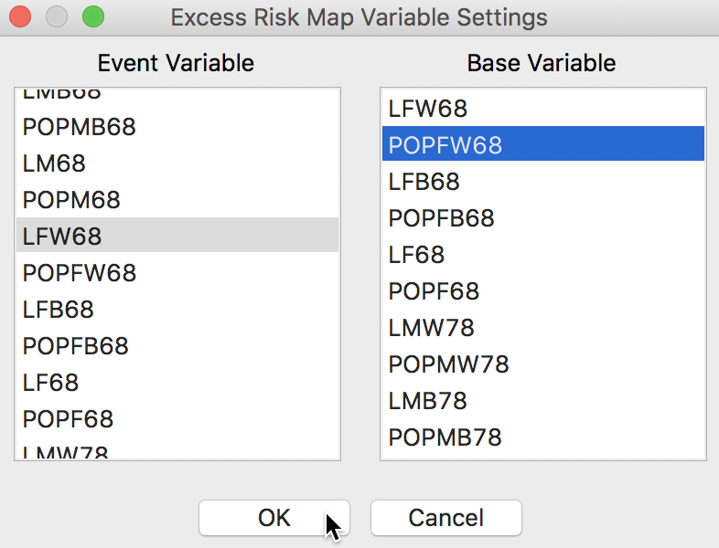
Figure 15: Excess Risk map variables
Clicking OK brings up the map shown in Figure 16.
In the excess risk map, the legend categories are hard coded, with the blue tones representing counties where the risk is less than the state average (excess risk ratio < 1), and the brown tones corresponding to those counties where the risk is higher than the state average (excess risk ratio > 1).
In the map in Figure 16, we have six counties with an SMR greater than 2 (the brown colored counties), suggesting elevated rates relative to the state average.
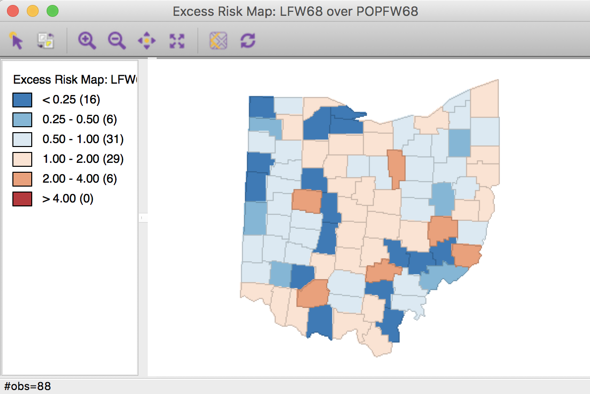
Figure 16: Excess Risk map
As before, all the usual options for a map are available. For example, we can save the categories as a new variable in the table.
Saving and calculating excess risk
In the same manner as for the raw rate map, we can save the excess risk results by means of the Save Rates map option. Since the excess risk map is hard coded with a particular legend, this is the only way to create other maps with the SMR as the underlying variable.
As soon as the rates are added to the table, they can then be used for any graph, map or other statistical analysis.
For example, using R_EXCESS (the suggested default variable name) as the variable name to save the rate to the table, we can create the box map in Figure 17. This map is identical to the box map for the crude rate in Figure 8.
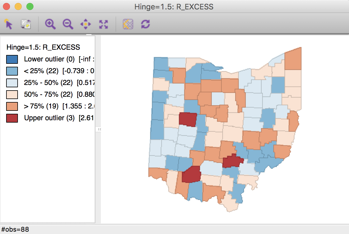
Figure 17: Box Map for SMR
Finally, to compare the extreme values suggested by the excess risk map and the box map for the relative risk, we select the category with SMR > 2 in the excess risk map (click on the corresponding brown box in the legend, as shown in the left-hand panel of Figure 18). As highlighted in the right-hand panel of Figure 18, it turns out that the box map applies a more stringent criterion to designate locations as having an elevated rate. The box map utilizes the full distribution of the rates to identify outliers, compared to the relative risk map, which identifies them as having a value greater than two.
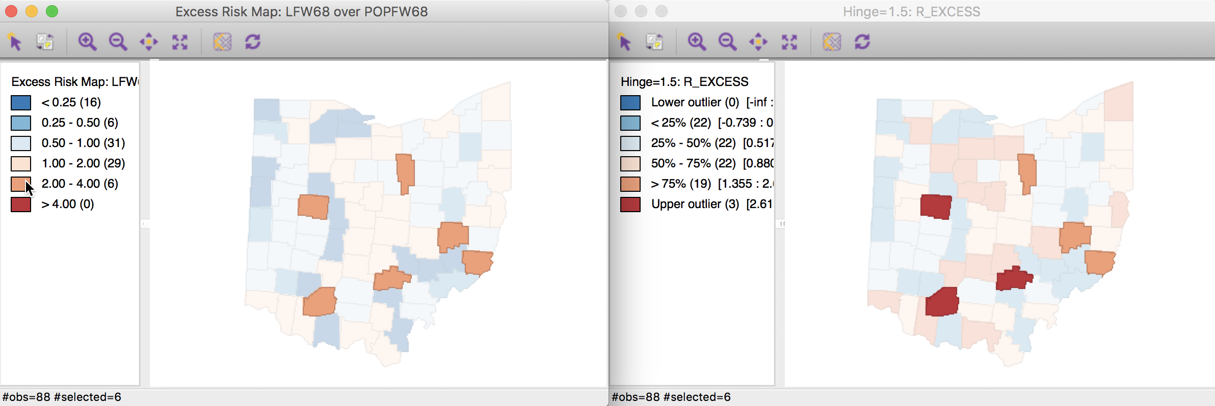
Figure 18: SMR outliers
As was the case for the crude rate, the excess risk can also be calculated by means of the table Calculator. This follows the same approach as for the raw rate, but requires the Excess Risk option, the second item in the drop down list of methods shown in Figure 12.
Empirical Bayes (EB) Smoothed Rate Map
Borrowing strength
As mentioned in the introduction, rates have an intrinsic variance instability, which may lead to the identification of spurious outliers. In order to correct for this, we can use smoothing approaches (also called shrinkage estimators), which improve on the precision of the crude rate by borrowing strength from the other observations. This idea goes back to the fundamental contributions of James and Stein (the so-called James-Stein paradox), who showed that in some instances biased estimators may have better precision in a mean squared error sense.
GeoDa includes three methods to smooth the rates: an Empirical Bayes approach, a spatial averaging approach, and a combination between the two. We will consider the spatial approaches after we discuss distance-based spatial weights. Here, we focus on the Empirical Bayes (EB) method. First, we provide some formal background on the principles behind smoothing and shrinkage estimators.
Bayes Law
The formal logic behind the idea of smoothing is situated in a Bayesian framework, in which the distribution of a random variable is updated after observing data. The principle behind this is the so-called Bayes Law, which follows from the decomposition of a joint probability (or density) into two conditional probabilities: \[ P[AB] = P[A | B] \times P[B] = P[B | A] \times P[A],\] where \(A\) and \(B\) are random events, and \(|\) stands for the conditional probability of one event, given a value for the other. The second equality yields the formal expression of Bayes law as: \[P[A | B] = \frac{P[B | A] \times P[A]}{P[B]}.\] In most instances in practice, the denominator in this expression can be ignored, and the equality sign is replaced by a proportionality sign:7 \[P[A | B] \propto P[B | A] \times P[A].\] In the context of estimation and inference, the \(A\) typically stands for a parameter (or a set of parameters) and \(B\) stands for the data. The general strategy is to update what we know about the parameter \(A\) a priori (reflected in the prior distribution \(P[A]\)), after observing the data \(B\), to yield a posterior distribution, \(P[A | B]\). The link between the prior and posterior distribution is established through the likelihood, \(P[B | A]\). Using a more conventional notation with say \(\pi\) as the parameter and \(y\) as the observations, this gives:8 \[P[\pi | y] \propto P[y | \pi] \times P[\pi].\]
The Poisson-Gamma model
For each particular estimation problem, we need to specify distributions for the prior and the likelihood in such a way that a proper posterior distribution results. In the context of rate estimation, the standard approach is to specify a Poisson distribution for the observed count of events (conditional upon the risk parameter), and a Gamma distribution for the prior of the risk parameter \(\pi\). This is referred to as the Poisson-Gamma model.9
In this model, the prior distribution for the (unknown) risk parameter \(\pi\) is Gamma(\(\alpha, \beta\)), where \(\alpha\) and \(\beta\) are the shape and scale parameters of the Gamma distribution. In terms of the more familiar notions of mean and variance, this implies: \[E[\pi] = \alpha / \beta,\] and \[Var[\pi] = \alpha / \beta^2.\] Using standard Bayesian principles, the combination of a Gamma prior for the risk parameter with a Poisson distribution for the count of events (\(O\)) yields the posterior distribution as Gamma(\(O + \alpha, P + \beta\)). The new shape and scale parameters yield the mean and variance of the posterior distribution for the risk parameter as: \[E[\pi] = \frac{O + \alpha}{P + \beta},\] and \[Var[\pi] = \frac{O + \alpha}{(P + \beta)^2}.\] Different values for the \(\alpha\) and \(\beta\) parameters (reflecting more or less precise prior information) will yield smoothed rate estimates from the posterior distribution. In other words, the new risk estimate adjusts the crude rate with parameters from the prior Gamma distribution.
The Empirical Bayes approach
In the Empirical Bayes approach, values for \(\alpha\) and \(\beta\) of the prior Gamma distribution are estimated from the actual data. The smoothed rate is then expressed as a weighted average of the crude rate, say \(r\), and the prior estimate, say \(\theta\). The latter is estimated as a reference rate, typically the overall statewide average or some other standard.
In essense, the EB technique consists of computing a weighted average between the raw rate for each county and the state average, with weights proportional to the underlying population at risk. Simply put, small counties (i.e., with a small population at risk) will tend to have their rates adjusted considerably, whereas for larger counties the rates will barely change.10
More formally, the EB estimate for the risk in location \(i\) is: \[\pi_i^{EB} = w_i r_i + (1 - w_i) \theta.\] In this expression, the weights are: \[w_i = \frac{\sigma^2}{(\sigma^2 + \mu/P_i)},\] with \(P_i\) as the population at risk in area \(i\), and \(\mu\) and \(\sigma^2\) as the mean and variance of the prior distribution.11
In the empirical Bayes approach, the mean \(\mu\) and variance \(\sigma^2\) of the prior (which determine the scale and shape parameters of the Gamma distribution) are estimated from the data.
For \(\mu\) this estimate is simply the reference rate (the same reference used in the computation of the SMR), \(\sum_{i=1}^{i=n} O_i / \sum_{i=1}^{i=n} P_i\). The estimate of the variance is a bit more complex: \[\sigma^2 = \frac{\sum_{i=1}^{i=n} P_i (r_i - \mu)^2}{\sum_{i=1}^{i=n} P_i} - \frac{\mu}{\sum_{i=1}^{i=n} P_i/n}.\] While easy to calculate, the estimate for the variance can yield negative values. In such instances, the conventional approach is to set \(\sigma^2\) to zero. As a result, the weight \(w_i\) becomes zero, which in essence equates the smoothed rate estimate to the reference rate.
EB rate map
An EB smoothed rate map is created from the map menu Rates-Calculated Map > Empirical Bayes. In the variable selection dialog, we again take LFW68 as the event variable and POPFW68 as the base variable. In the drop down list of map types, we choose a Box Map (Hinge=1.5), as shown in Figure 19.
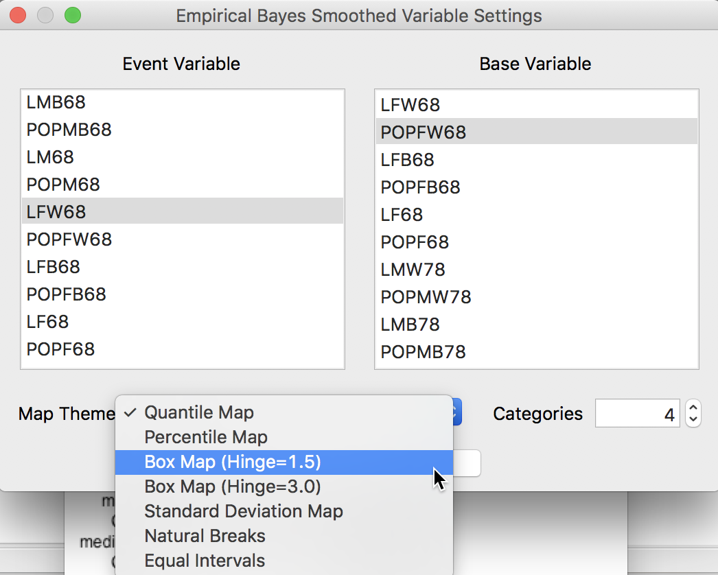
Figure 19: EB map variables
Clicking OK brings up the map in Figure 20.
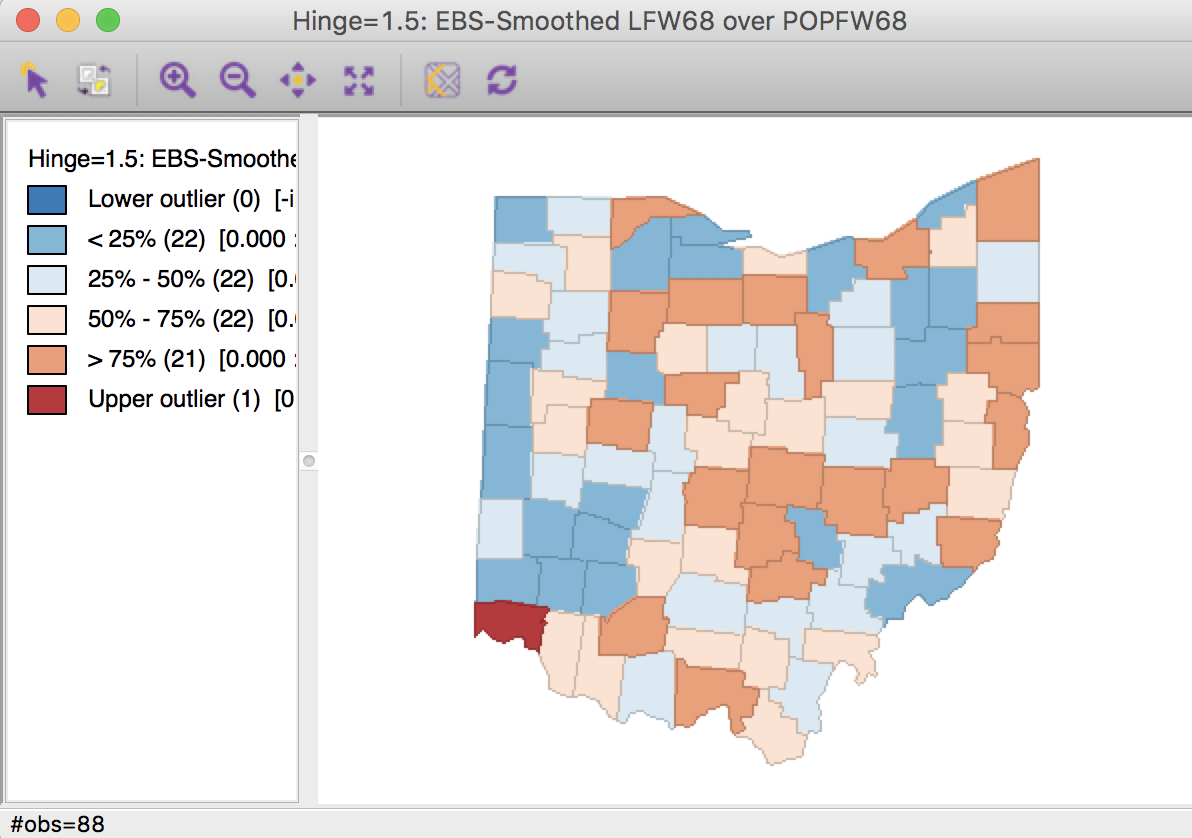
Figure 20: EB rate map
In comparison to the box map for the crude rates and the excess rate map, none of the original outliers remain identified as such in the smoothed map. Instead, a new outlier is shown in the very southwestern corner of the state (Hamilton county).
Since many of the original outlier counties have small populations at risk (check in the data table), their EB smoothed rates are quite different (lower) from the original. In contrast, Hamilton county is one of the most populous counties (it contains the city of Cincinnati), so that its raw rate is barely adjusted. Because of that, it percolates to the top of the distribution and becomes an outlier.
To illustrate this phenomenon, we can systematically select observations in the box plot for the raw rates and compare their position in the box plot for the smoothed rates. This will reveal which observations are affected most.
We create the box plots in the usual way, but make sure to select Save Rates first to add the EB smoothed rate to the table (as R_EBS). We also want to use View > Set Display Precision on Axes to have more meaningful tick points (the default of 2 yields all rates as 0.00).
For example, as shown in Figure 21, we can place the box plot for the crude rate RLFW68 next to the box plot for the EB-smoothed rates (R_EBS). We select the three outliers in the box plot to the right. The corresponding observations are within the upper quartile for the EB smoothed rates, but well within the fence, and thus no longer outliers after smoothing. We can of course also locate these observations on the map, or any other open views.
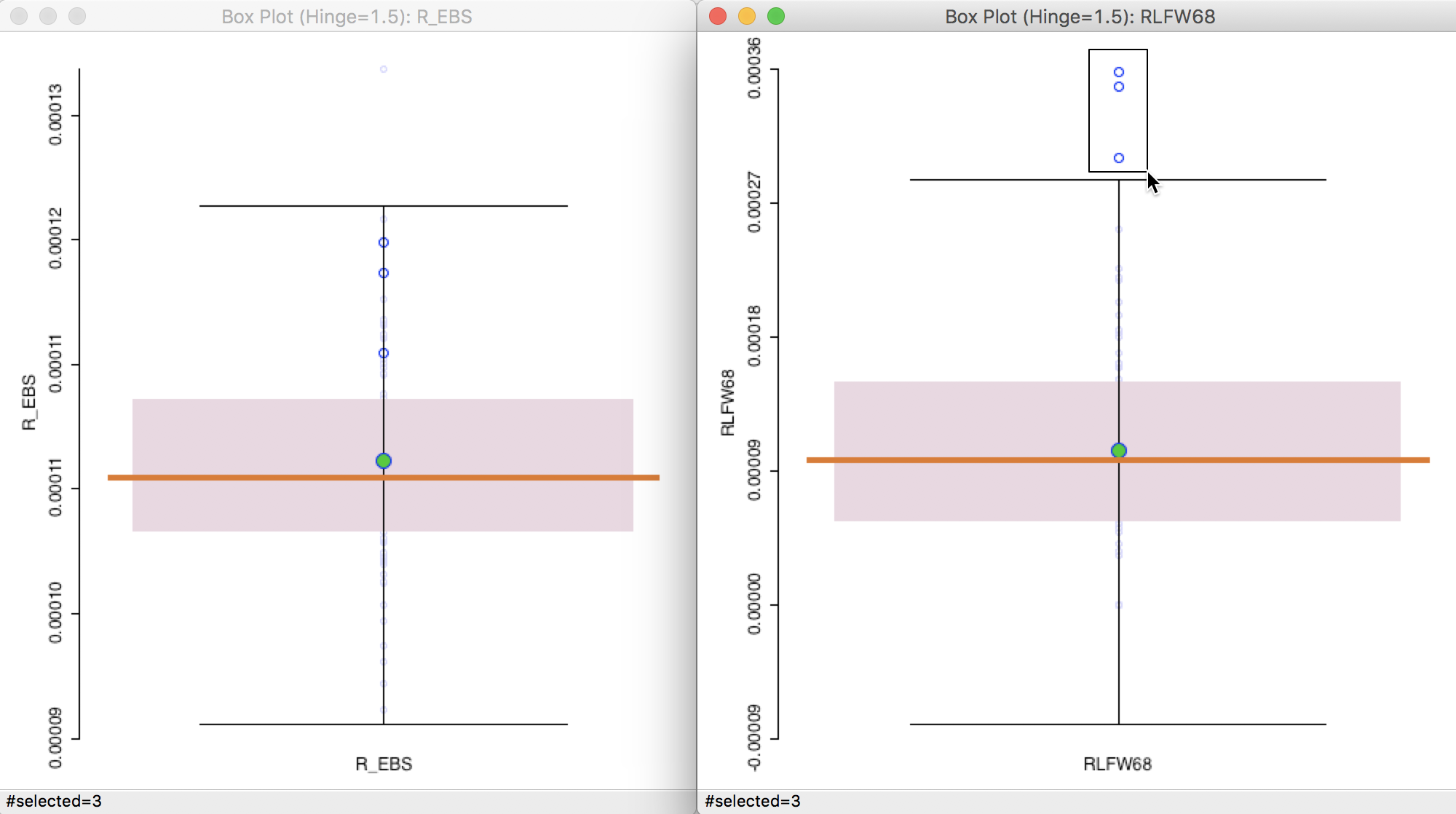
Figure 21: Outliers for crude rate vs EB rate
Next, we can carry out the reverse and select the outlier in the box plot for the EB smoothed rate, as in the left-hand panel of Figure 22. Its position is around the 75 percentile in the box plot for the crude rate. Also note how the range of the rates has shrunk. Many of the higher crude rates are well below 0.00012 for the EB rate, whereas the value for the EB outlier has barely changed.
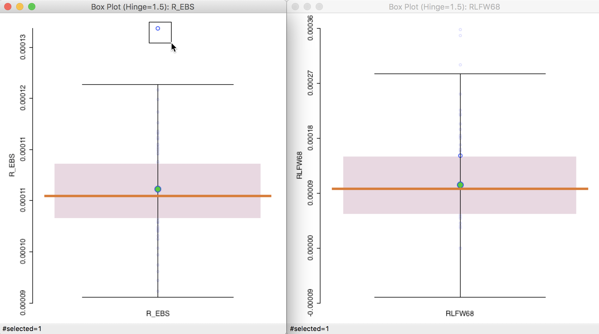
Figure 22: Outliers for EB rate vs crude rate
References
Anselin, Luc, Nancy Lozano-Gracia, and Julia Koschinky. 2006. “Rate Transformations and Smoothing.” Technical Report. Urbana, IL: Spatial Analysis Laboratory, Department of Geography, University of Illinois.
Clayton, David, and John Kaldor. 1987. “Empirical Bayes Estimates of Age-Standardized Relative Risks for Use in Disease Mapping.” Biometrics 43:671–81.
Gelman, Andrew, John B. Carlin, Hal S. Stern, David B. Dunson, Aki Vehtari, and Donald B. Rubin. 2014. Bayesian Data Analysis, Third Edition. Boca Raton, FL: Chapman & Hall.
Lawson, Andrew B., William J. Browne, and Carmen L. Vidal Rodeiro. 2003. Disease Mapping with WinBUGS and MLwiN. Chichester: John Wiley.
Marshall, R. J. 1991. “Mapping Disease and Mortality Rates Using Empirical Bayes Estimators.” Applied Statistics 40:283–94.
Xia, Hong, and Bradley P. Carlin. 1998. “Spatio-Temporal Models with Errors in Covariates: Mapping Ohio Lung Cancer Mortality.” Statistics in Medicine 17:2025–43.
-
University of Chicago, Center for Spatial Data Science – anselin@uchicago.edu↩
-
For example, see Xia and Carlin (1998) and Lawson, Browne, and Rodeiro (2003).↩
-
In actuality, this is a little trickier than advertised. The best way is to first search for utm zone 17, then select SR-ORG:13 WGS 1984 UTM Zone 17N. At that point, google it and then click on the link for EPSG:32617.↩
-
We get this result by viewing the number of events as a draw of \(O_i\) events from a population of size \(P_i\). This follows a binomial distribution with parameter \(\pi\) (the proportion of events in the population). The mean of this distribution is \(\pi P_i\) and the variance is \(\pi (1 - \pi) P_i\). A little algebra yields the result that the mean of the rate \(O_i/P_i\) is \(\pi P_i / P_i = \pi\), confirming the unbiasness of the crude rate as an estimator for the underlying risk. The variance is \(\pi (1 - \pi) P_i / P_i^2 = \pi (1 - \pi) / P_i\).↩
-
Note that the current version of GeoDa does not support age-adjusted rates, which are common practice in epidemiology.↩
-
Also specify after last variable (at the bottom of the variables list) next to the insert before option to replicate the table screen shot in Figure 14.↩
-
There are several excellent books and articles on Bayesian statistics, with Gelman et al. (2014) as a classic reference.↩
-
Note that in a Bayesian approach, the likelihood is expressed as a probability of the data conditional upon a value (or distribution) of the parameters. In classical statistics, it is the other way around.↩
-
For an extensive discussion, see, for example, the classic papers by Clayton and Kaldor (1987) and Marshall (1991).↩
-
For an extensive technical discussion, see also Anselin, Lozano-Gracia, and Koschinky (2006).↩
-
In the Poisson-Gamma model, this turns out to be the same as \(w_i = P_i / (P_i + \beta)\).↩