Spatial Weights as Distance Functions
Luc Anselin1
03/17/2018 (revised and updated)
Introduction
In this Chapter, we consider two situations where the values for the spatial weights take on a special meaning. The weights are transformations of the original distances. The two examples covered consist of inverse distance functions and kernel weights.
The resulting weights files primarily provide the basis for creating new spatially explicit variables for use in further analyses, such as in spatial regression specifications.2 The weights themselves are not used in measures of spatial autocorrelation or other exploratory analyses in GeoDa, where only the existence of a neighbor relation is taken into account.
We will illustrate this functionality with the data set that we used earlier for point locations of house sales for Cleveland, OH.
Objectives
-
Compute inverse distance functions
-
Compute kernel weights functions
-
Assess the characteristics of weights based on distance functions
-
Understand the contents of KWT format weights files
GeoDa functions covered
- Weight File Creation dialog
- inverse distance weights
- kernel weights
- bandwidth options
- diagonal element options
Getting started
We will again use the data set that contains the location and sales price of 205 homes in a core area of Cleveland, OH for the fourth quarter of 2015. We get started by clearing the previous project and dropping the file clev_sls_154_core.shp into the Drop files here rectangle of the connect to data source dialog. Alternatively, we can use a project file if we saved one earilier (e.g., clev_sls_154_core.gda). The familiar themeless base map results, as in Figure 1.
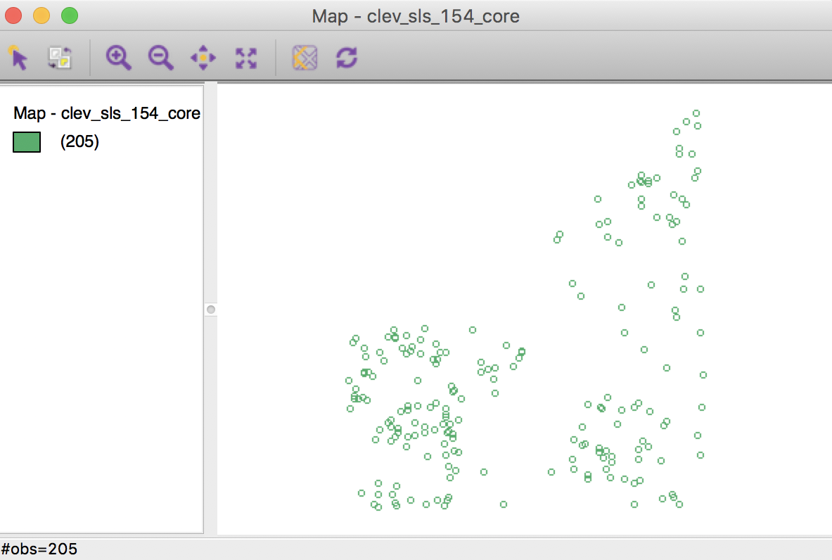
Figure 1: Cleveland home sales themeless map
If desired, we can again add the base layer and change the point colors and selection default. We pass on this for now.
Inverse Distance Weights
Concepts
One can readily view spatial weights based on a distance cut-off as representing a step function, with a value of 1 for neighbors with \(d_{ij} < \delta\), and a value of 0 for others. As before, \(d_{ij}\) stands for the distance between observations \(i\) and \(j\), and \(\delta\) is the bandwidth.
A straightforward extension of this principle is to consider a continuous parameterized function of distance itself: \[\begin{equation} w_{ij} = f(d_{ij},\mathbf{\theta}), \end{equation}\] with \(f\) as a functional form and \(\mathbf{\theta}\) a vector of parameters.
In order to conform to Tobler’s first law of geography, a distance decay effect must be respected.3 In other words, the value of the function of distance needs to decrease with a growing distance. More formally, the partial derivative of the distance function with respect to distance should be negative, \(\partial w_{ij} / \partial d_{ij} < 0\).
Commonly used distance functions are the inverse, with \(w_{ij} = 1 / d_{ij}^{\alpha}\) (and \(\alpha\) as a parameter), and the negative exponential, with \(w_{ij} = e^{-\beta d_{ij}}\) (and \(\beta\) as a parameter). The functions are often combined with a distance cut-off criterion, such that \(w_{ij} = 0\) for \(d_{ij} > \delta\).
In practice, the parameters are seldom estimated, but typically set to a fixed value, such as \(\alpha = 1\) for inverse distance weights (\(1/d_{ij}\)), and \(\alpha = 2\) for gravity weights (\(1/d_{ij}^{2}\)). By convention, the diagonal elements of the spatial weights are set to zero and not computed. Plugging in a value of \(d_{ii} = 0\) would yield division by zero for inverse distance weights.
The distance-based weights depend not only on the parameter value and functional form, but also on the metric used for distance. Since the weights are inversely related to distance, large values for the latter will yield small values for the former, and vice versa. This may be a problem in practice when the distances are so large (i.e., measured in small units) that the corresponding inverse distance weights become close to zero, possibly resulting in a zero spatial weights matrix.
In addition, a potential problem may occur when the distance metric is such that distances take on values less than one. As a consequence, some inverse distance values may be larger than one, which is typically not a desired result.
Rescaling of the coordinates will fix both problems.
Creating inverse distance functions for distance bands
We proceed in the usual fashion to create spatial weights based on an inverse distance function. In the Weights File Creation interface, we specify unique_id as the ID variable, and select the Distance Weight option.
As before, we choose Distance band from the three types of weights. The default bandwidth of 3598.055030 is the same as encountered previously. We keep it as is for now. The inverse distance option is invoked by the check box below the bandwidth entry, as in Figure 2. For now, we keep the Power value to its default of 1.
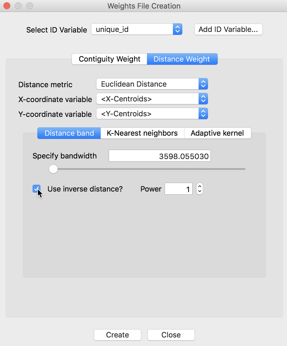
Figure 2: Inverse distance option
Clicking on the Create button results in the usual query for a file name specification. The inverse distance weights are saved in a file with a GWT extension, say clev_sls_154_core_id1.gwt.
Properties of inverse distance weights
As soon as the file is created, the properties of the weights appear in the weights manager, as illustrated in Figure 3.
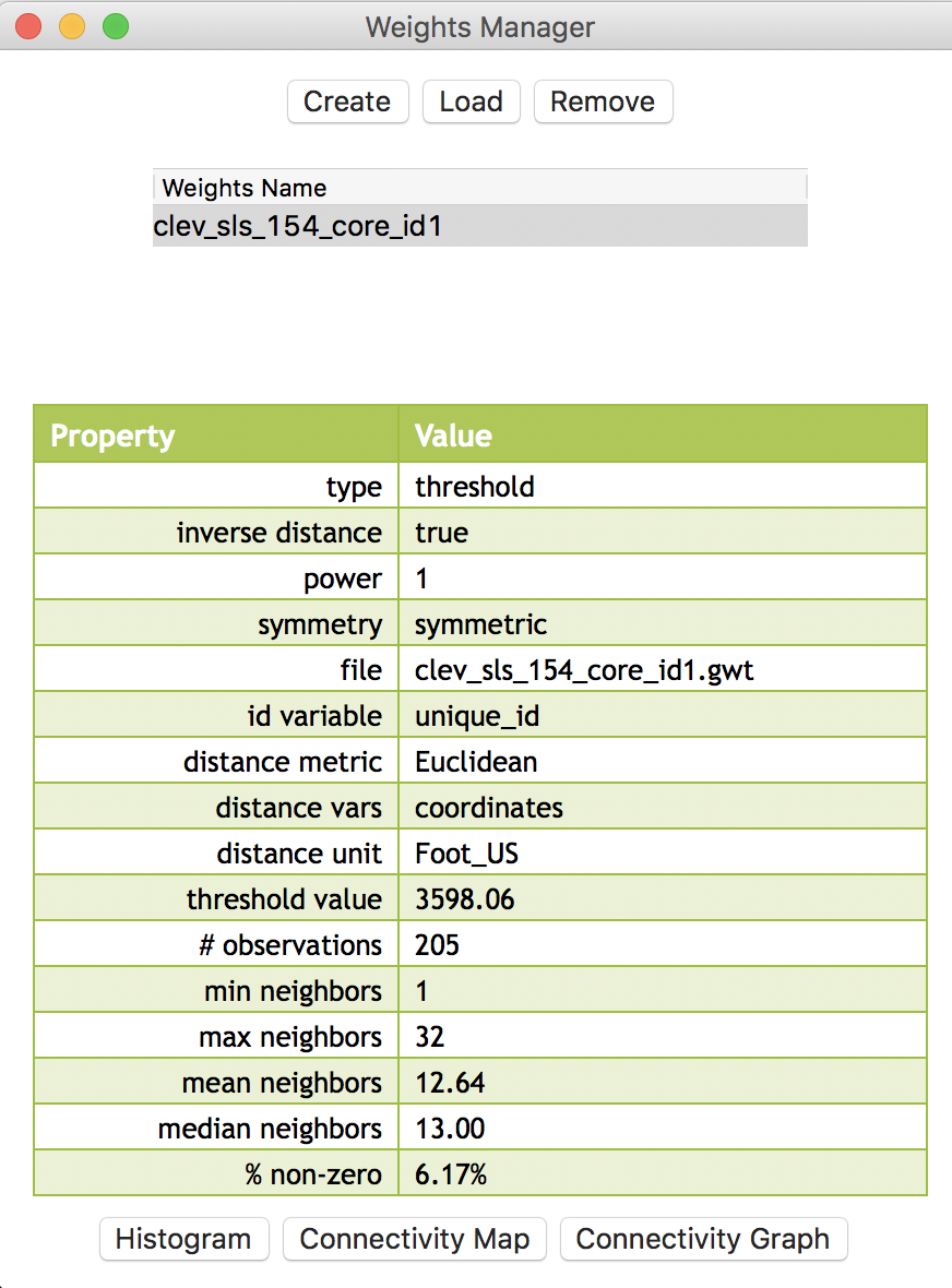
Figure 3: Inverse distance weights properties
Since the properties only pertain to the connectivity structure implied by the weights, they are identical to the ones obtained for the standard distance-band weights. It is important to keep in mind that the actual values for the weights are ignored in this operation. The only differences between the two property lists are the listing of inverse distance as true, and the value for power as 1.
The connectivity map and the connectivity graph associated with the weights are the same as before as well. For example, the connectivity graph shown in Figure 4 is identical to the one we obtained for the distance-band weights.
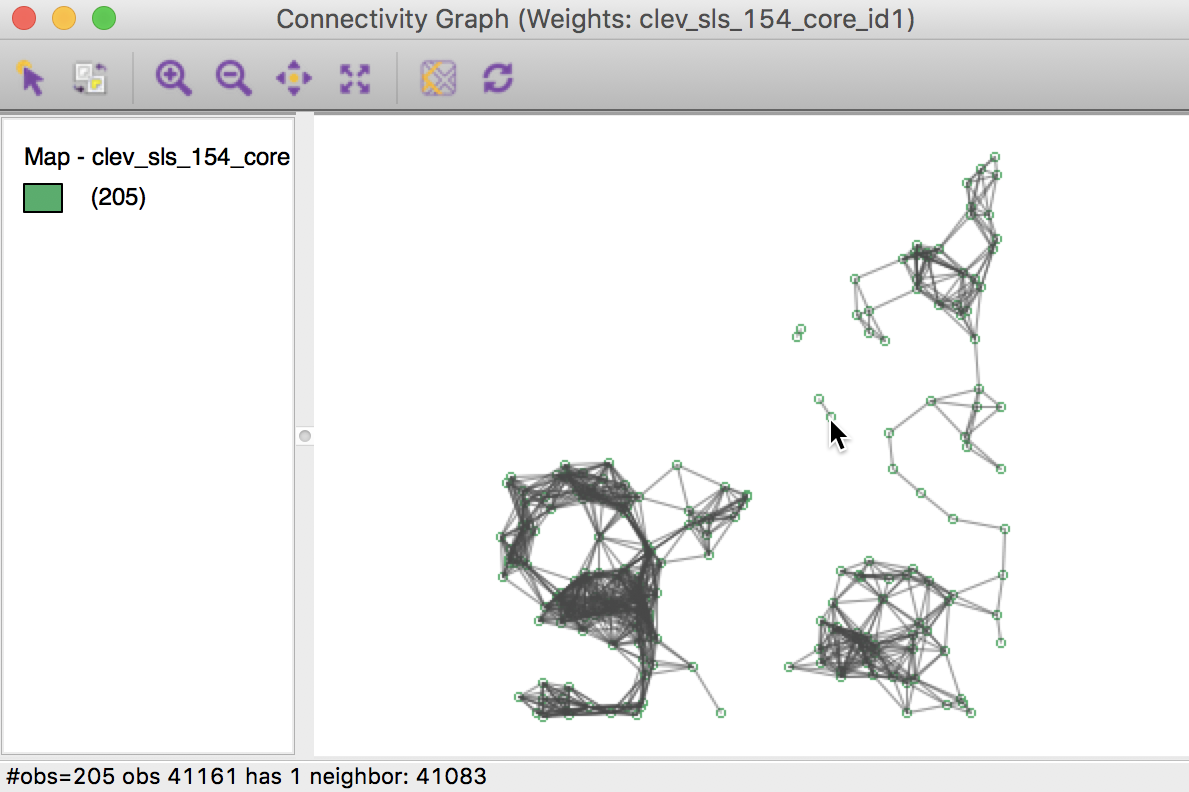
Figure 4: Connectivity graph for inverse distance weights
The default bandwidth is such that each location is ensured to have at least one neighbor, but as we have seen before, this can be changed. This allows inverse distance weights to be calculated for any bandwidth specified. For example, if the bandwidth is set as the maximum inter-point distance, the resulting weights will be for a full matrix. This is not recommended for larger data sets, but it can provide a useful point of departure to compute various accessibility indices.4
Inverse distance weights in the GWT file
Figure 5 provides a comparison of the entries in the GWT file for respectively the distance-band weights and the inverse distance weights. We notice that the pairs of neighbors are identical, as expected. Also, the value for the inverse distance weight is exactly the inverse of the distance.
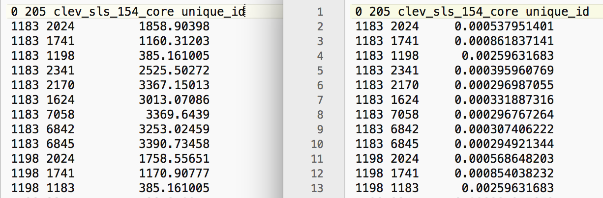
Figure 5: GWT file for distance band and inverse distance weights
Using non-geographical coordinates
So far, we have been using the default setting of <X-Centroids> and <Y-Centroids> for the coordinates that were the input into the distance calculations. However, this option is perfectly general, and any two variables contained in the data set can be specified as x, y coordinates. For example, this allows for the computation of so-called socio-economic weights, where the difference between two locations on any two variables can be used as the distance metric.5
We illustrate this feature in Figure 6, where we explicitly specify the x and y coordinates as the variables x and y (the sample data set does not include any other meaningful variables besides the house price). Also, we compute inverse distance squared by setting the Power parameter to 2.
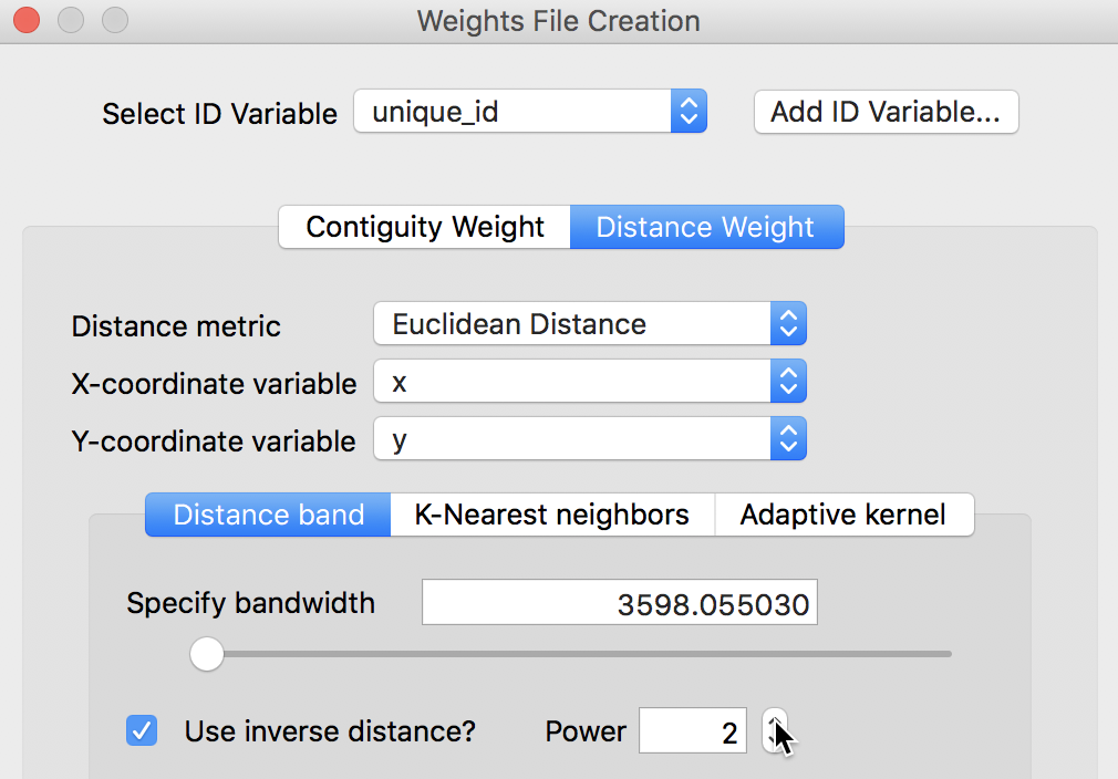
Figure 6: Inverse distance for generic coordinates
The contents of the resulting GWT file are shown in Figure 7. This highlights the problem alluded to above, i.e., that the value of the weights critically depends on the distance metric. In our example, the second power of the inverse distances result in weights that are essentially not distinguishable from zero.
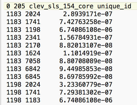
Figure 7: Inverse squared distance in GWT file
Note that since the connectivity properties ignore the actual weights, they will again not differ from the ones obtained for the matching distance-band weights. However, any calculation of spatially explicit variables using these weights (e.g., a spatially lagged variable) would be largely meaningless, since the spatially lagged variables would all roughly equal zero. The importance of this potential problem cannot be stressed enough, since a mechanical computation using these weights could lead to very misleading results in further analyses.
Creating inverse distance functions for k-nearest neighbors
Computing inverse distance weights is not limited to a distance band specification. As shown in Figure 8, the inverse distance option is also available for K-Nearest neighbors.
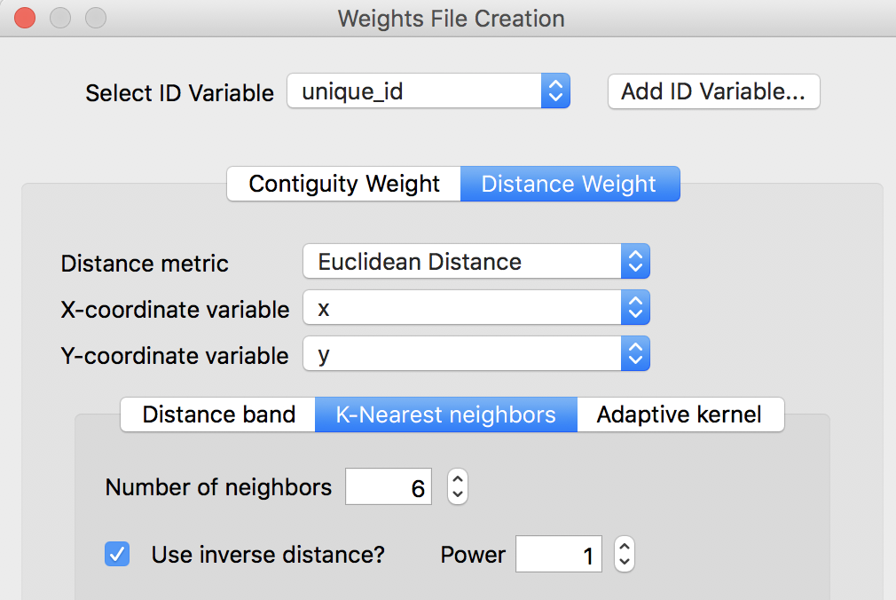
Figure 8: Inverse distance for k-nearest neighbors
This option works in the same way as for the distance bands. With the Number of neighbors and a Power specified, the new weights are computed from the distances between the k nearest neighbors for each location. In Figure 9, the original k-nearest distances (with k=6, as specified in Figure 8) and the corresponding inverse weights entries are shown from the respective GWT files.
Figure 9: GWT file for KNN and associated inverse distance weights
As is the case for the inverse distance band weights, the actual values of the inverse knn weights are ignored in further spatial analyses in GeoDa. They can only be used in the calculation of spatially explicit variables.6
Kernel Weights
Concepts
Kernel weights are used in non-parametric approaches to model spatial covariance, such as in the HAC method for heteroskedastic and spatial autocorrelation consistent variance estimates.7 In GeoDa, kernel functions can be computed, but as is the case for the other distance functions, the actual values of the weights are only used in the computation of spatially explicit variables.
The kernel weights are defined as a function \(K(z)\) of the ratio between the distance \(d_{ij}\) from \(i\) to \(j\), and the bandwidth \(h_i\), with \(z = d_{ij} / h_i\). This ensures that \(z\) is always less than 1. For distances greater than the bandwidth, \(K(z) = 0\).
Five different kernel weights functions are currently supported:
- Uniform, \(K(z) = 1/2\) for \(|z| < 1\),
- Triangular, \(K(z) = (1 - |z| )\) for \(|z| < 1\),
- Quadratic or Epanechnikov, \(K(z) = (3/4) (1 - z^2)\) for \(|z| < 1\),8
- Quartic, \(K(z) = (15/16)(1 - z^2)^2\) for \(|z| < 1\), and
- Gaussian. \(K(z) = (2 \pi)^{(1/2)} \exp(- z^2 / 2)\).9
Typically, the value for the diagonal elements of the weights is set to 1, although GeoDa allows for the actual kernel value to be used as well.
Many careful decisions must be made in selecting a kernel weights function. Apart from the choice of a functional form for \(K(\ )\), a crucial aspect is the selection of the bandwidth. In the literature, the latter is found to be more important than the functional form.
A drawback of fixed bandwidth kernel weights is that the number of non-zero weights can vary considerably, especially when the density of the point locations is not uniform throughout space. This is the same problem encountered for the distance band spatial weights.
In GeoDa, there are two types of fixed bandwidths for kernel weights. One is the max-min distance used earlier (the largest of the nearest-neighbor distances). The other is the maximum distance for a given specification of k-nearest neighbors. For example, with knn set to a given value, this is the distance between the selected k-nearest neighbors pairs that are the farthest apart.
To correct for the issues associated with a fixed bandwidth, a variable bandwidth approach adjusts the bandwidth for each location to ensure equal or near-equal coverage. One common approach is to take the k-nearest neighbors, and to adjust the bandwidth for each location such that exactly k neighbors are included in the kernel function. The bandwidth specific to each location is then any distance larger than its k nearest neighbor distance, but less than the k+1 nearest neighbor distance.
In GeoDa, the default value for k equals the cube root of the number of observations (following the recommendation in Kelejian and Prucha 2007). In general, a wider bandwidth gives smoother and more robust results, so the bandwidth should always be set at least as large as the recommended default.
Creating kernel weights
We create kernel weights in the by now familiar fashion, by selecting the Adaptive kernel option under the Distance Weight button of the Weights File Creation dialog. Figure 10 illustrates the five kernel functions that are available.
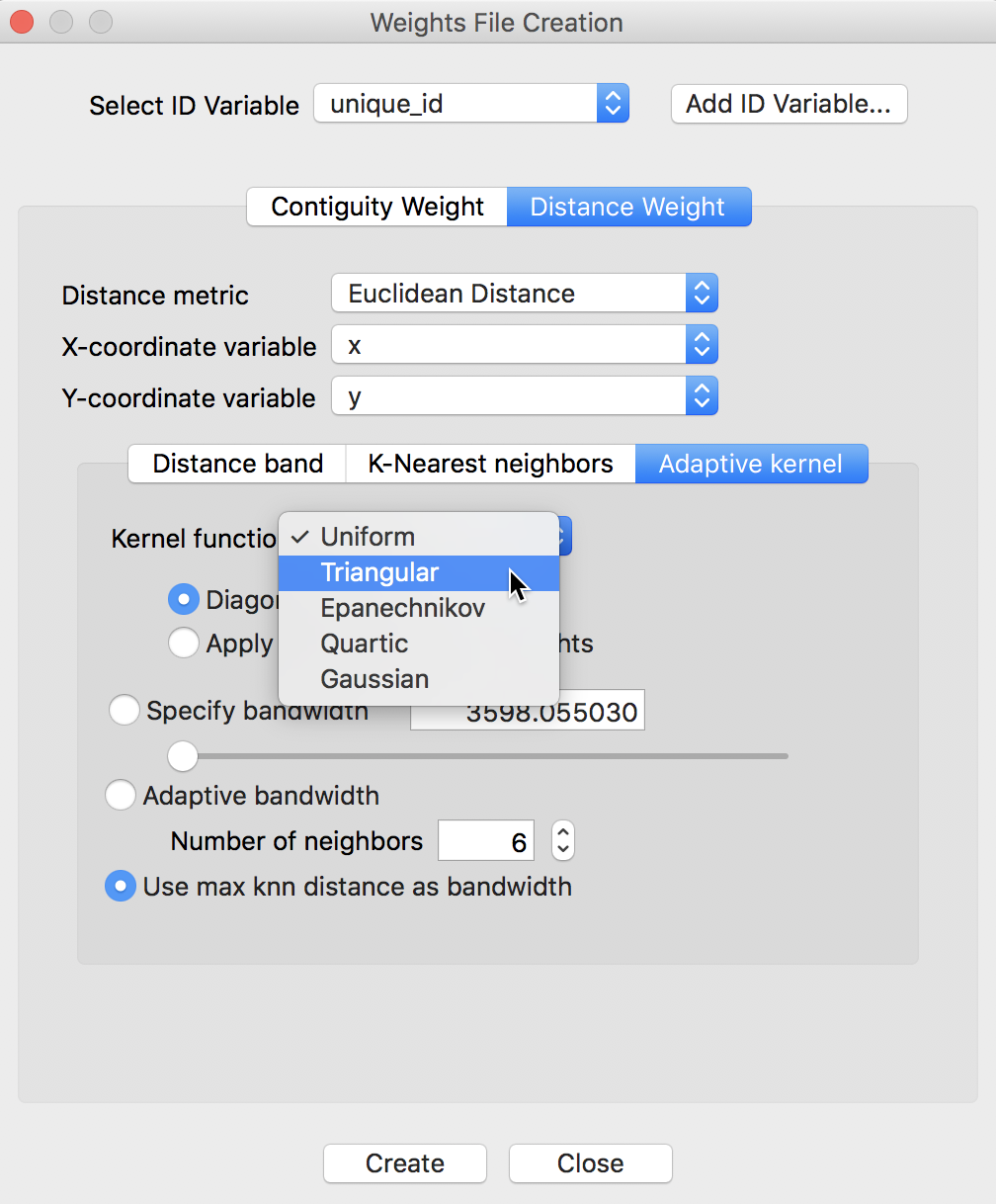
Figure 10: Kernel weight options
To illustrate this functionality, we select the Triangular option, with the Adaptive bandwidth set to the default number of neighbors of 6. We also leave the Diagonal weights option to its default of 1 (i.e., the kernel function is not applied to a distance of zero for the diagonal elements). These settings are illustrated in Figure 11.
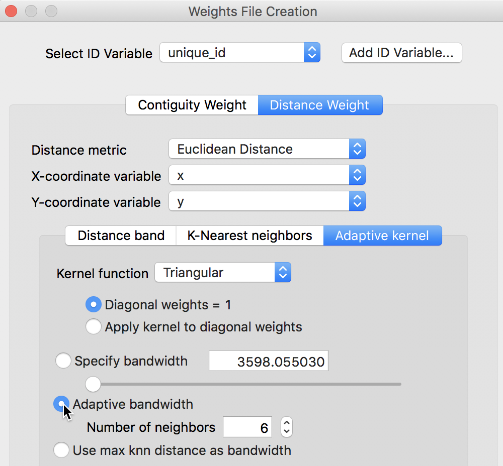
Figure 11: Triangular adaptive kernel
The results are saved in a file with file extension KWT (such as clev_sls_154_core_tri6.kwt). The KWT file extension is adopted to retain compatibility with the conventions assumed for PySAL and its spreg module, as implemented in GeoDaSpace. Except for the inclusion of the diagonal element, its structure is the same as a GWT format file.
The contents of the KWT file in our example are shown in the right-hand panel of Figure 12, compared to the knn distances in the corresponding GWT file on the left.
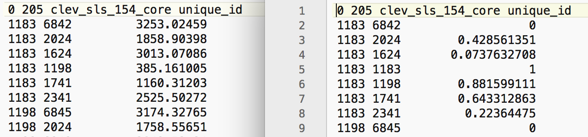
Figure 12: KWT file for triangular adaptive kernel
A few characteristics of the results should be noted. First, the bandwidth is determined by the largest distance among the six neighbors. In the current example, for the first observation considered (with unique_id 1183), this is the distance given on the first row. The distance between 1183 and 6842 amounts to 3253.02459, as shown in the left panel of Figure 12. By convention, each other distance is converted to a value less than one by dividing it by this maximum distance.
For example, for the second pair (between 1183 and 2024), this would yield 1858.90398/3253.02459 = 0.571439 (the \(z\)-value referred to above). The result for the triangular kernel is then 1 - 0.571439 = 0.428561, i.e., the value shown on the second line of the KWT file.
For the pair with the largest distance, the value of the kernel is zero (1 - 1). Finally, for the diagonal element (the pair 1183, 1183), the kernel is given as 1, by construction.10
Properties of kernel weights
As soon as the weights are created, their properties appear in the weights manager. As illustrated in Figure 13, the descriptive statistics are again the same as for standard knn weights. The differences are in the first six items. The type of weights is given as kernel, the kernel method is identified (triangular), with the bandwidth definition (knn 6) and adptive kernel set to true. It is also indicated that the kernel is not applied to the diagonal elements (kernel to diagonal is false). Also, as for the knn weights, the resulting weights are asymmetric. These items will be saved to a project file when one is created.
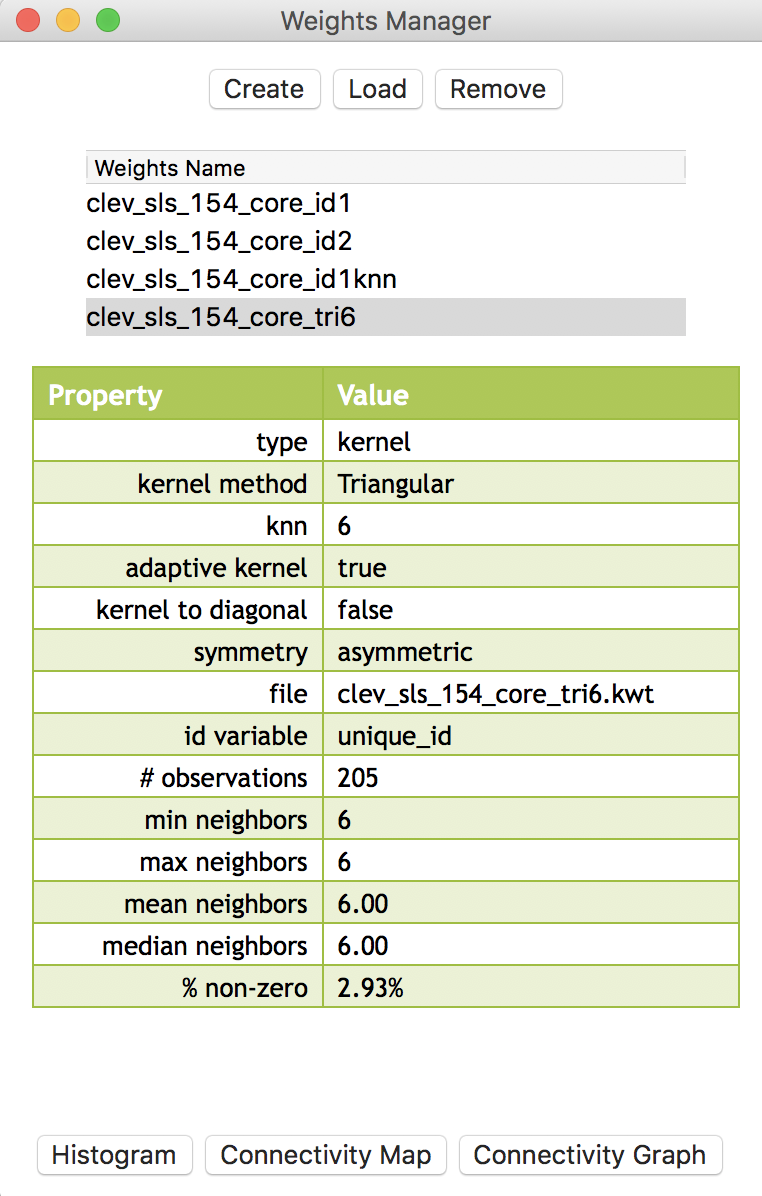
Figure 13: Triangular adaptive kernel properties
Since the connectivity histogram, map and graph ignore the actual weights values and are solely based on the implied connectivity structure, they are identical to those obtained for the corresponding knn weights. For example, Figure 14 showns the connectivity graph, which is the same as generated in the previous Chapter.
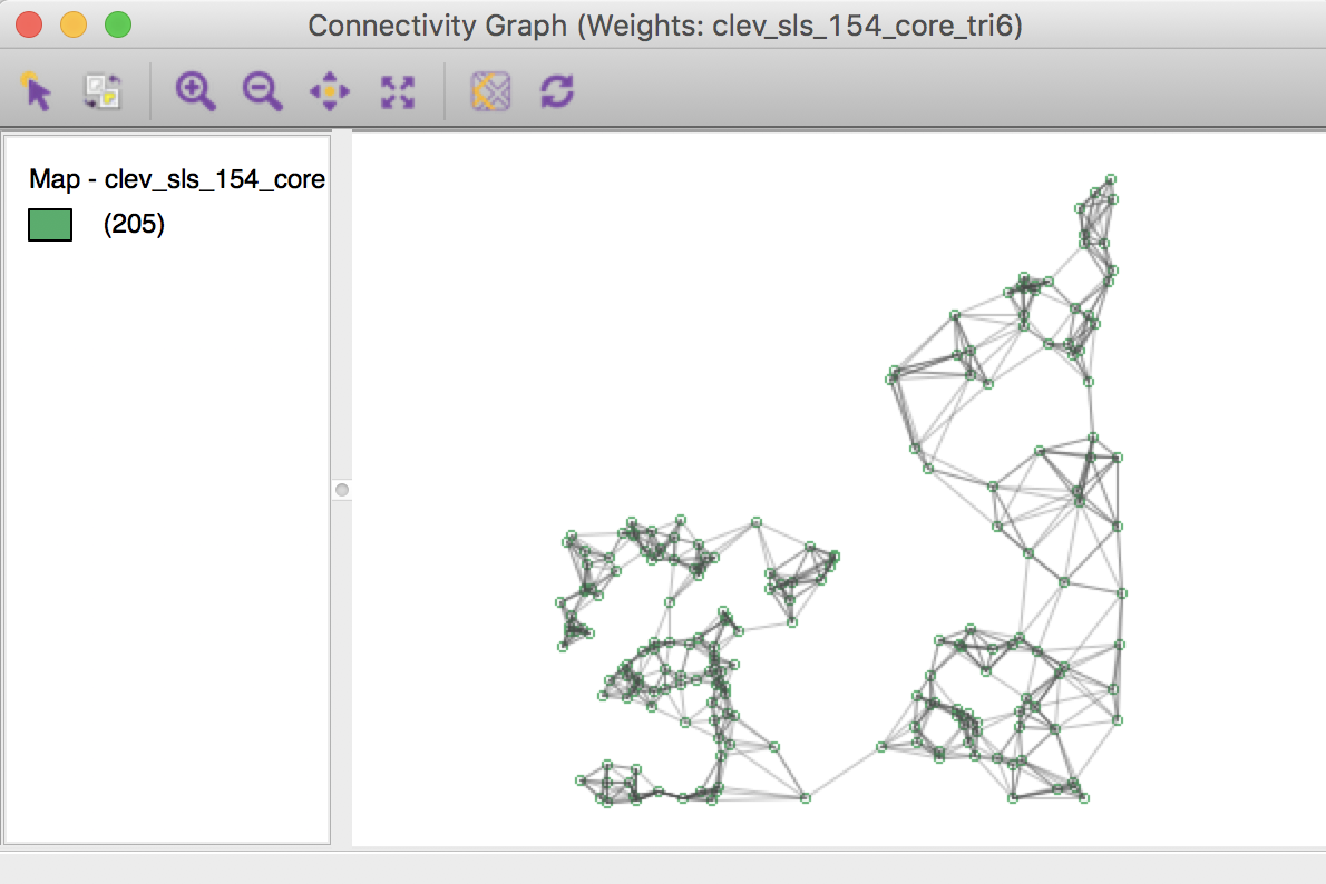
Figure 14: Connectivity graph for triangular kernel weights
Treatment of diagonal elements
As mentioned, for a triangular kernel, the diagonal elements equal one, irrespective of the setting for that option. To illustrate the effect of applying the kernel function to the diagonal elements, we choose the Epanechnikov option, as shown Figure 15. The Apply kernel to diagonal weights radio button is selected as well.
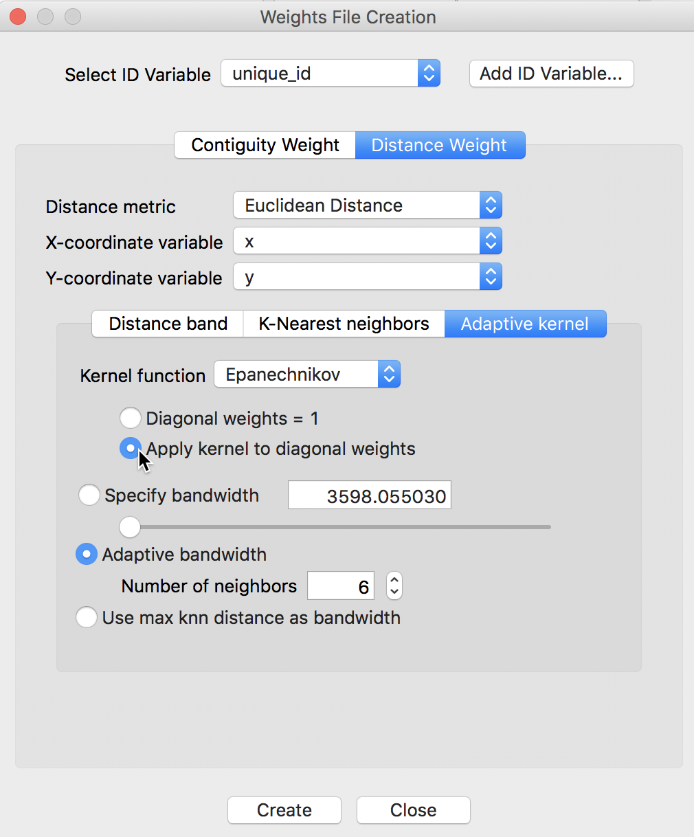
Figure 15: Epanechnikov kernel with diagonal option
All other options are the same as before. The contents of the resulting KWT file, again compared to the knn GWT file, are shown in Figure 16.
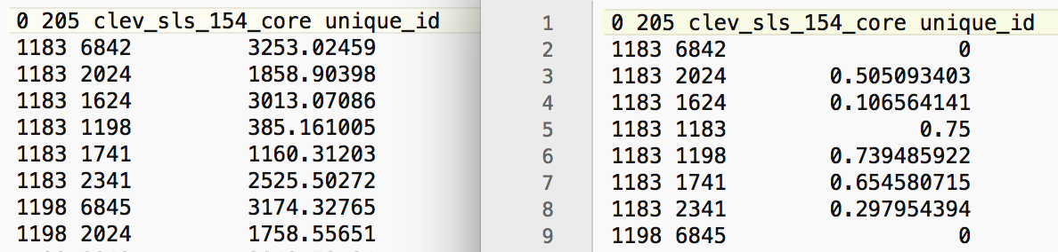
Figure 16: KWT file for Epanechnikov adaptive kernel
As before, the value for the most separated points is zero, but now the diagonal elements equal 0.75, which results from the 3/4 scaling factor being applied to 1. In all other respects, these weights are treated in the same way as the others discussed in this Chapter.
References
Anselin, Luc, and Sergio J. Rey. 2014. Modern Spatial Econometrics in Practice, a Guide to Geoda, Geodaspace and Pysal. Chicago, IL: GeoDa Press.
Hall, P., and P. Patil. 1994. “Properties of Nonparametric Estimators of Autocovariance for Stationary Random Fields.” Probability Theory and Related Fields 99:399–424.
Kelejian, Harry H., and Ingmar R. Prucha. 2007. “HAC Estimation in a Spatial Framework.” Journal of Econometrics 140:131–54.
Tobler, Waldo. 1970. “A Computer Movie Simulating Urban Growth in the Detroit Region.” Economic Geography 46:234–40.
-
University of Chicago, Center for Spatial Data Science – anselin@uchicago.edu↩
-
The distance functions in GeoDa provide an alternative and more user-friendly way to calculate the weights included in PySAL and GeoDaSpace (see Anselin and Rey 2014 for details).↩
-
Tober’s so-called first law of geography postulates that everything is related to everything else, but closer things more so (Tobler 1970).↩
-
Specific measures of accessibility are currently not explicitly supported in GeoDa. However, in some instances, the calculation of a spatially lagged variables using spatial weights with inverse distances (squared) between all the pairs of observations may be a meaningful measure of accessibility, as discussed in the next Chapter.↩
-
For socio-economic distances to be meaningful, one has to be mindful of the scale in which those variables are expressed. One useful application that we will encounter in a later chapter is to use the coordinates obtained from a multi-dimensional scaling exercise as the input for distance computations. Also, the current implementation in GeoDa is limited to two dimensions, and multi-attribute distance measures are not supported.↩
-
Both inverse distance band and inverse distance knn weights can be used as inputs in the spatial regression analyses implemented in GeoDaSpace and PySAL (see Anselin and Rey 2014, for specifics).↩
-
This method is currently not implemented in GeoDa, but is available in GeoDaSpace and PySal (see Hall and Patil 1994; Kelejian and Prucha 2007, among others, for technical aspects, and Anselin and Rey (2014), for implementation details).↩
-
Note that the Epanechnikov kernel is sometimes referred to without the (3/4) scaling factor. GeoDa implements the scaling factor.↩
-
While the Gaussian kernel is in principle without a bandwidth constraint, in GeoDa it is implemented with the same bandwidth option as the other kernel functions.↩
-
For this case, it turns out that the calculated kernel value is also one, since 1 - 0 = 1.↩