Objectives

• Create a spatially lagged variable as an average or sum of the neighbors

• Create a spatially lagged variable as a window sum or average

• Create a spatially lagged variable based on inverse distance weights

• Create a spatially lagged variable based on kernel weights

• Rescaling coordinates to obtain inverse distance weights

• Compute and map spatially smoothed rates

• Compute and map spatial Empirical Bayes smoothed rates

Getting started

To start, we continue to use the data set that contains the location and sales price of 205 homes in a core area of Cleveland, OH for the fourth quarter of 2015. We also need to have several spatial weights active in the weights manager. At the very least, we need k-nearest neighbor weights for k=6, inverse distance weights using the k-nearest neighbors with k=6, and Epanechnikov kernel weight, again using the adaptive kernel for k=6 nearest neighbors, and with the kernel applied to the diagonal weights (the diagonals will thus equal 0.75). We can either create these weights in the current project (after dropping the file clev_sls_154_core.shp into the Drop files here rectangle of the connect to data source dialog), or load a project file that contains the weights.

In the example shown in Figure 1, the three weights files are clev_sls_154_core_k6 (for knn contiguity), clev_sls_154_core_k6id (for inverse distance applied to the k=6 nearest neighbors), and clev_sls_154_core_k6epadiag (for the Epanechnikov kernel weights). Figure 1 highlights the properties of the latter, as listed in the weights manager (note how the kernel to diagonal is set to true).

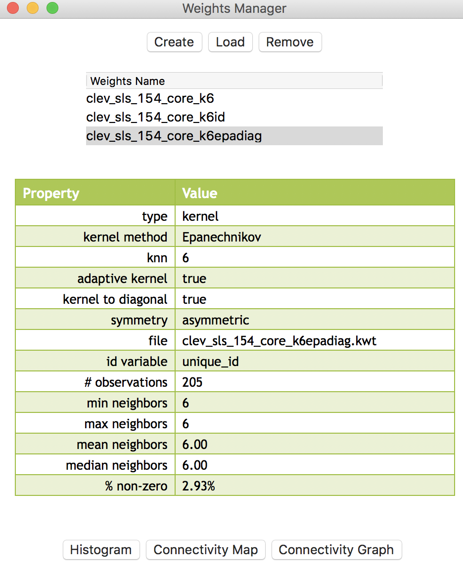
Figure 1: Spatial weights for Cleveland point data

Concept

With a neighbor structure defined by the non-zero elements of the spatial weights matrix \(\mathbf{W}\), a spatially lagged variable is a weighted sum or a weighted average of the neighboring values for that variable. In most commonly used notation, the spatial lag of \(y\) is then expressed as \(Wy\).

Formally, for observation \(i\), the spatial lag of \(y_i\), referred to as \([Wy]_i\) (the variable \(Wy\) observed for location \(i\)) is: \[\begin{equation*} [Wy]_i = w_{i1}y_1 + w_{i2}y_2 + \dots + w_{in}y_n, \end{equation*}\] or, \[\begin{equation*} [Wy]_i = \sum_{j=1}^n w_{ij}y_j, \end{equation*}\] where the weights \(w_{ij}\) consist of the elements of the \(i\)-th row of the matrix \(\mathbf{W}\), matched up with the corresponding elements of the vector \(\mathbf{y}\).

In other words, the spatial lag is a weighted sum of the values observed at neighboring locations, since the non-neighbors are not included (those \(i\) for which \(w_{ij} =0\)). Typically, the weights matrix is very sparse, so that only a small number of neighbors contribute to the weighted sum. For row-standardized weights, with \(\sum_j w_{ij} = 1\), the spatially lagged variable becomes a weighted average of the values at neighboring observations.

In matrix notation, the spatial lag expression corresponds to the matrix product of the \(n \times n\) spatial weights matrix \(\mathbf{W}\) with the \(n \times 1\) vector of observations \(\mathbf{y}\), or \(\mathbf{W \times y}\). The matrix \(\mathbf{W}\) can therefore be considered to be the spatial lag operator on the vector \(\mathbf{y}\).

In a number of applied contexts, it may be useful to include the observation at location \(i\) itself in the weights computation. This implies that the diagonal elements of the weights matrix must be non-zero, i.e., \(w_{ii} \neq 0\). Depending on the context, the diagonal elements may take on the value of one or equal a specific value (e.g., for kernel weights where the kernel function is applied to the diagonal). We will highlight this issue in the specific illustrations that follow.

Creating a spatially lagged variable

In GeoDa, the spatial lag computation is carried out through the Calculator dialog activated from the table menu (Table > Calculator), and selecting the Spatial Lag tab. The Weight drop down list contains all the spatial weights available to the project, with the currently active weights listed. In the example illustrated in Figure 2, we use the contiguity defined by knn with 6 nearest neighbors, contained in the clev_sls_154_core_k6 weights.

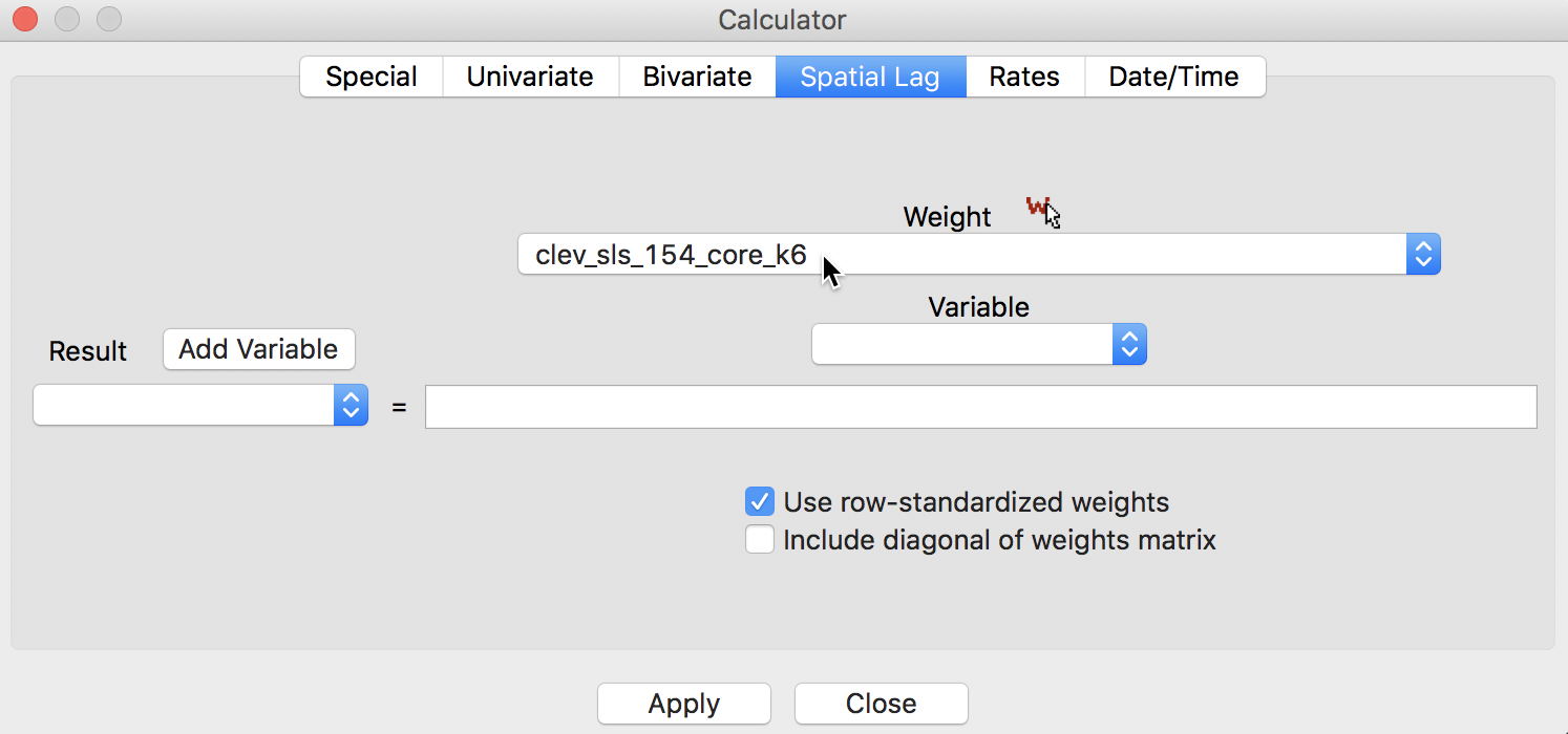
Figure 2: Spatial Lag tab in calculator

The process we follow is the usual one for creating new variables. We first Add a variable to the table and then initiate the particular computation to Apply to the variable. We next go over the four alternatives available through the interface.

Spatial lag with row-standardized weights

The default case is to Use row-standardized weights and to not include the diagonal weights (i.e., the observation itself) in the computation. For example, we can Add a variable LAG1 (and include it after the last variable in the table). Next, we apply the spatial lag operation to the variable sale_price, as shown in Figure 3.

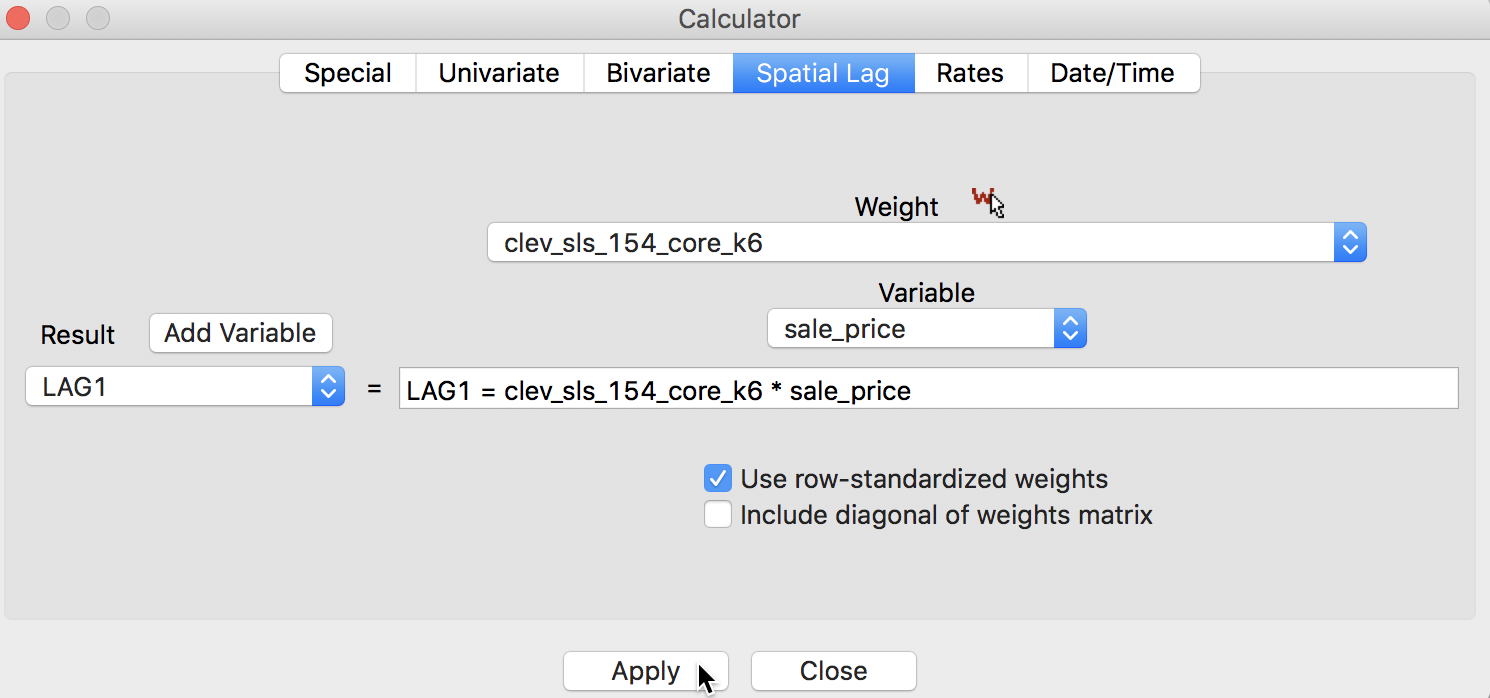
Figure 3: Spatial Lag for sales price

After clicking on Apply, the new variable is entered into the table, as illustrated in Figure 4. In order to make it a little easier to compare the various computations, we moved the column for unique_id and sale_price over to the right, and placed them right next to the spatial lag, LAG1.

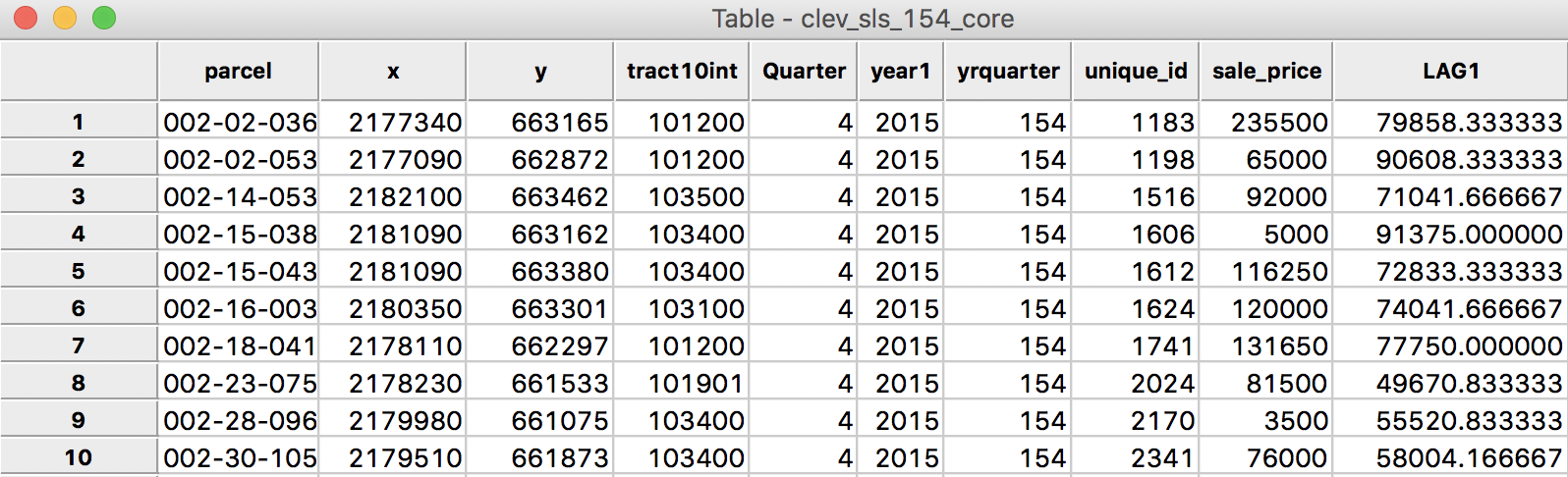
Figure 4: Spatial Lag for sales price in table

We quickly verify this operation by identifying the neighbors for the first location (with unique_id 1183) from the entries in the corresponding GWT file. As shown in Figure 5, the six locations in question are those with unique_id 6842, 2024, 1624, 1198, 1741, and 2341.²

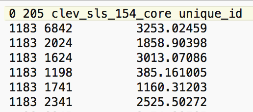
Figure 5: Neighbors for location 1183

We can also find the associated sales prices in the table (use the Selection Tool on the unique_id to find the relevant observations). They are listed in Figure 6, with the sales price for location 1183 on the first row.

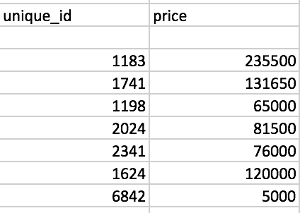
Figure 6: Sales price for neighbors of location 1183

We now verify the value for the spatial lag listed in the table. It is obtained as the average of the sales price for the six neighbors, or (131650 + 65000 + 81500 + 76000 + 120000 + 5000)/6 = 79858.33.

We can quickly assess the effect of the spatial averaging by comparing the descriptive statistics between the original price variable and its spatial lag (for example, by viewing the descriptive statistics associated with a histogram or box plot graph). The typical effect of the spatial lag is a compression of the range and variance of the variable. The range goes from $1,049 to $527,409 for the original variable to $6,583-$229,583 for the spatial lag. Similarly, the standard deviation is considerably reduced from 60,654 to 36,464.

A more dramatic view of the influence of high-valued or low-valued neighbors on the spatial lag is given by the PCP. In several instances in the graph shown in Figure 7, the line goes from a high price to a much lower spatial lag, and vice versa. In other words, if there is high spatial heterogeneity in the data, the choice of the neighborhood (the spatial weights) becomes very important, and the spatial lag may not be a good proxy for the value observed at a given location (recall that the value at the given location is not included in the spatial lag calculation). This relates directly to the notion of local spatial autocorrelation that we will examine in a later chapter.

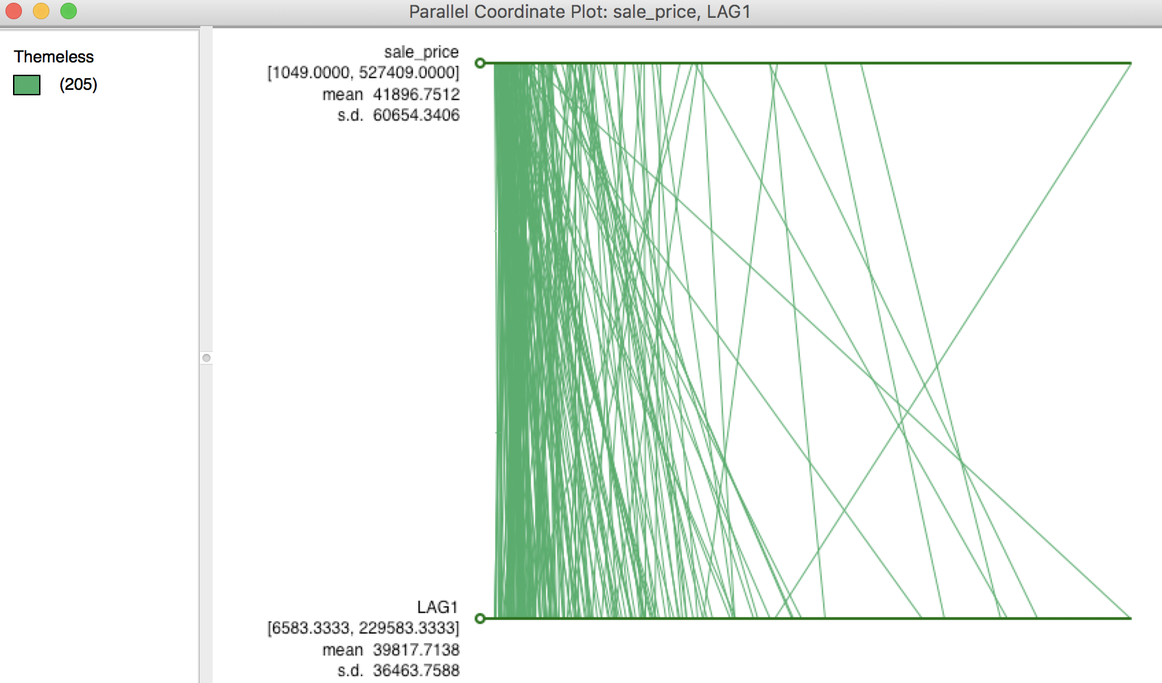
Figure 7: PCP for sales price and its spatial lag

Spatial lag as a sum of neighboring values

The default in GeoDa is to apply the spatial weights in row-standardized form. Hence the box associated with User row-standardized weights in Figure 3 is checked by default. In some applications (for example, when dealing with 0-1 observations), one may be interested in the spatial lag computed with the original binary weights (i.e., without applying row-standardization). This is accomplished by unchecking the default box, as in Figure 8.³

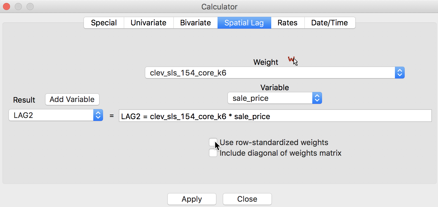
Figure 8: Spatial Lag sum for sales price

The result is as shown in the table in Figure 9.

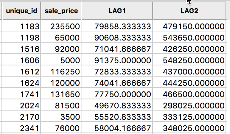
Figure 9: Spatial Lag sum for sales price in table

A quick check using the values from the table in Figure 6, reveals the lag sum for observation 1183 as 131650 + 65000 + 81500 + 76000 + 120000 + 5000 = 479150.

In the case of knn weights, there may be some value in comparing the lag sums across observations. After all, since the number of neighbors is constant, these values are nothing but the original spatial lags scaled by a factor of k (i.e., six in our example). However, it is important to note that in most applications, the number of neighbors will not be constant across observations, in which case the sums will no longer be comparable.

In the special case where the variable of interest is binary (0-1), the spatial lag sum will indicate the number of neighboring locations with an observation equal to 1. This is useful for computing join count statistics for local spatial autocorrelation, which we will consider in a later chapter.

Spatial window average

A third notion of spatial lag based on the concept of connectivity is that of a spatial window average. This includes the value at the observation itself in the computation of the average. This option is invoked by checking both the Use row-standardized weights and the Include diagonal of weights matrix boxes in the interface, as illustrated in Figure 10.

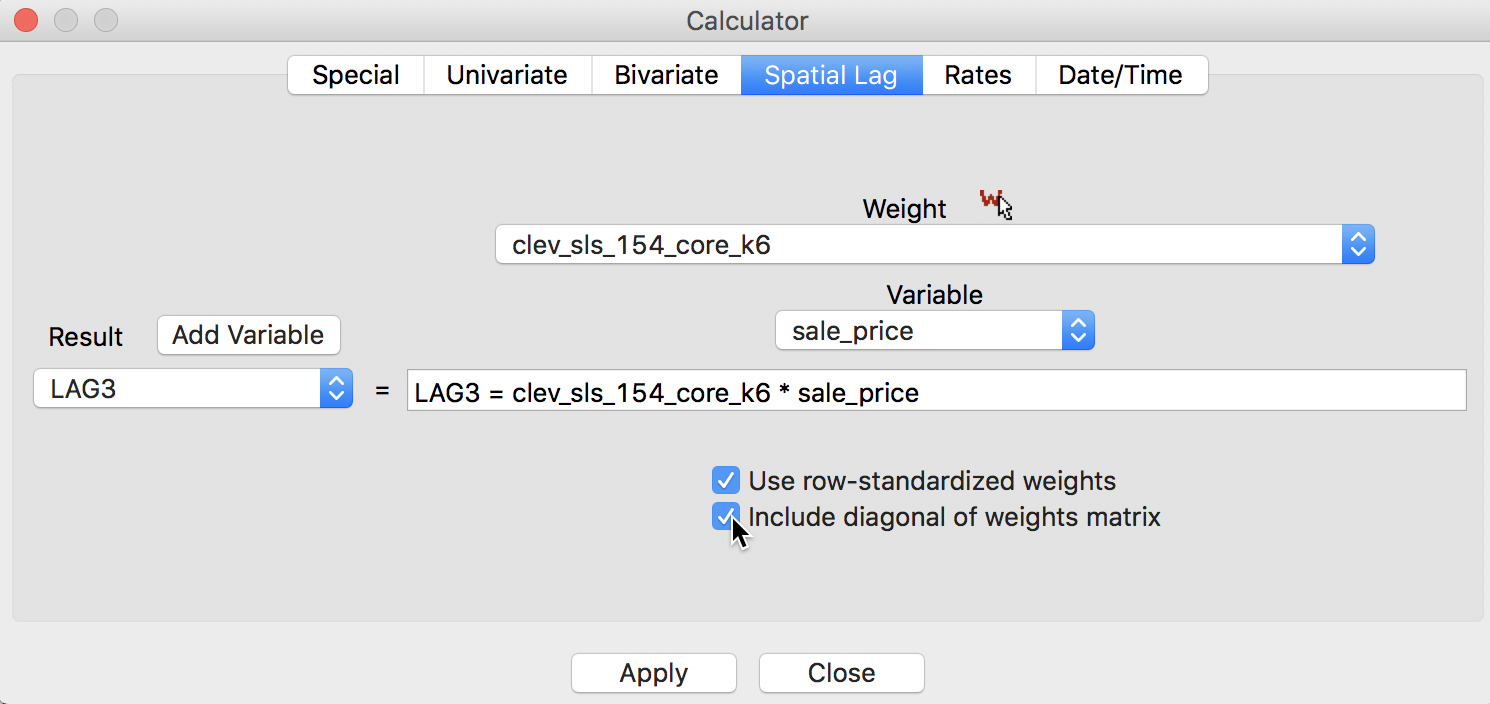
Figure 10: Spatial window average for sales price

The result is inlcuded in our example table as variable LAG3, as shown in Figure 11.

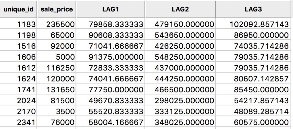
Figure 11: Spatial window average for sales price in table

In this calculation, the value for the location 1183 is the average of seven values, (235500 + 131650 + 65000 + 81500 + 76000 + 120000 + 5000)/7 = 102092.86.

Spatial window sum

Finally, we have the spatial window sum, the counterpart of the window average, but without using row-standardized weights. The corresponding box in the interface is thus unchecked, as in Figure 12, but the Include diagonal of weights matrix is maintained.

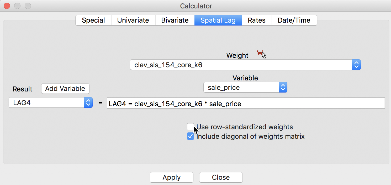
Figure 12: Spatial window sum for sales price

The new variable LAG4 is added to the table as in Figure 13.

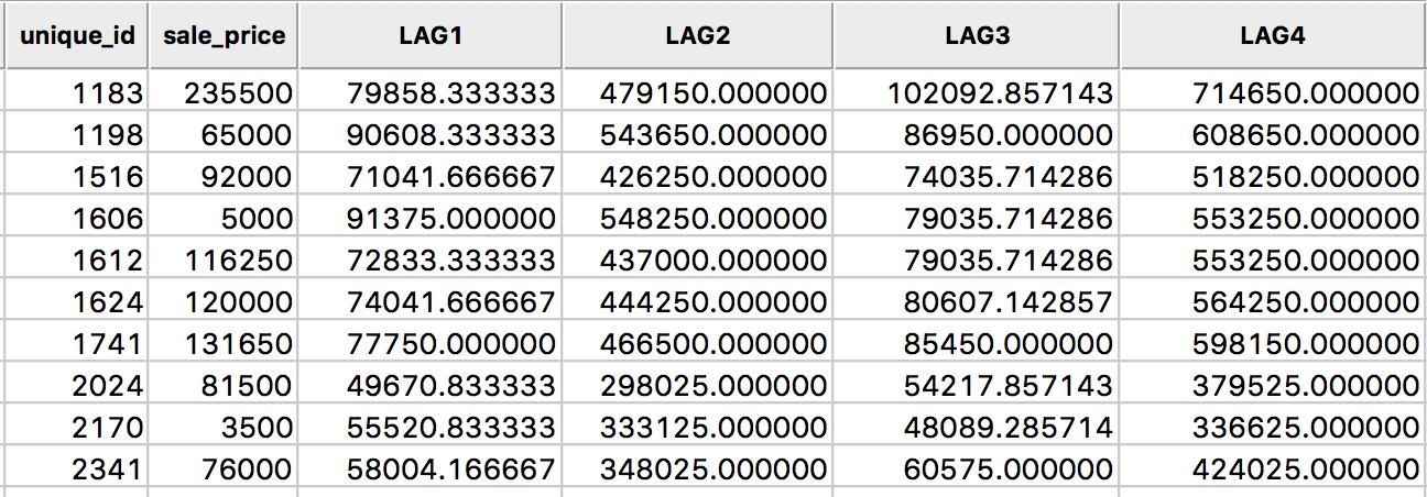
Figure 13: Spatial window sum for sales price in table

The spatial window sum is simply the sum of the sales price for the observation at 1183 and its six neighbors, or, 235500 + 131650 + 65000 + 81500 + 76000 + 120000 + 5000 = 714650. As in the case of the spatial lag sum, the spatial window sum may not be comparable among observations when the number of neighbors varies (for knn weights, the same number of neighbors is enforced by construction). When dealing with a binary variable, the spatial window sum corresponds to the number of events (observations with a value of 1) within the window centered on a location (including the value at that location).

Spatially lagged variables from inverse distance weights

Default setting

In contrast to the default setting for other weights, the preferred option for inverse distance weights is to keep the original values for the weights and not row-standardize, as illustrated in Figure 14, with the two check boxes unchecked. Note how the selected weight is clev_sls_154_core_k6id, the inverse distance weights from our example. This selection triggers the particular default settings for the check boxes.

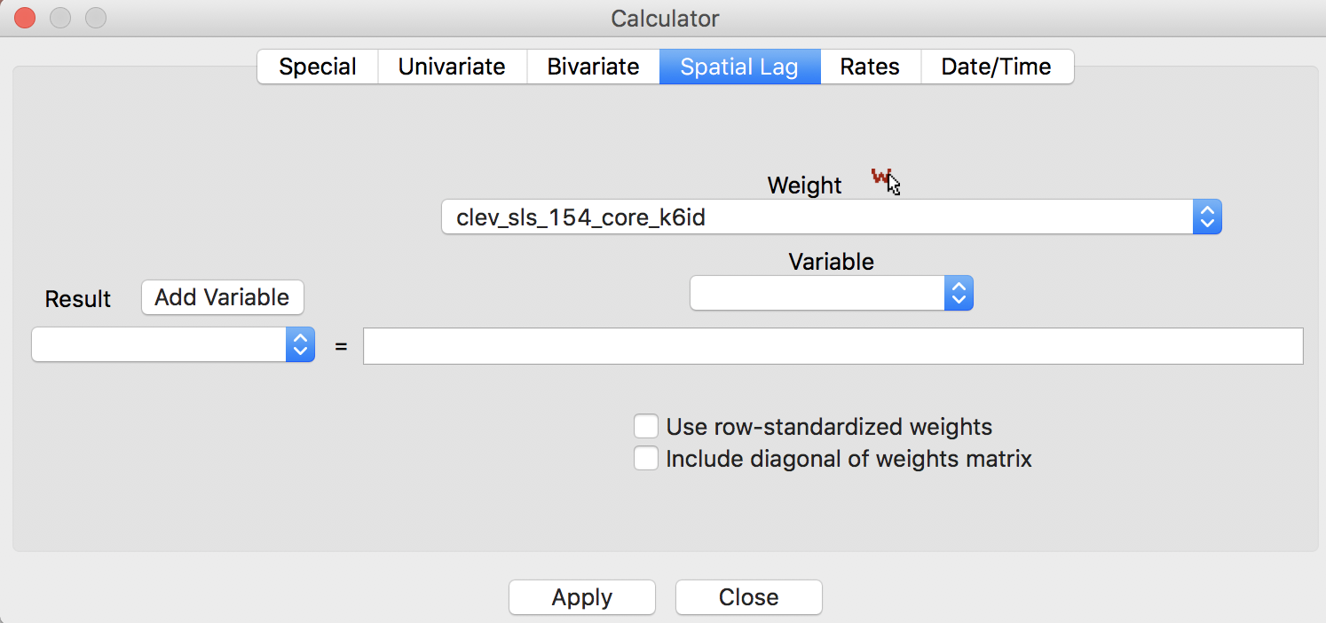
Figure 14: Inverse distance lag default options

In all other respects, the lag computation proceeds in the same way as for connectivity weights. In the first step, a new variable is added to the table, followed by the actual calculation.

The results of the various options are given in the four right-most columns of the table shown in Figure 15. The default case, with row-standardized weights off and no diagonal elements, is shown as the variable IDNRND. Compared to the original sales price, the lagged values are quite different. This is due to the scale of the inverse distance weights (the largest of which is 0.0026, see also Figure 16).

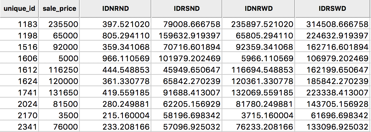
Figure 15: Inverse distance spatial lags for sales price in table

The third column, IDNRWD, shows the results when the diagonal is included (i.e., with the diagonal weights check box selected). This amounts to the value in IDNRND augmented by the sales price. For example, for the observation with unique_id 1183, the result is 397.521 + 235500 = 235897.521. This is equivalent to: \[[Wy]_i = y_i + \sum_j \frac{y_j}{d_{ij}^\alpha}.\] In some contexts, this may be the desired result, but it is by no means the most intuitive concept. It should therefore be used sparingly and only when there is a strong substantive motivation.

Spatial lags with row-standardized inverse distance weights

The original inverse distance weights are highly scale dependent. This can be remedied by expressing them in row-standardized form. The spatial lag then takes on the standard meaning of a weighted average of the values at neighboring observations. The main difference with lags computed for connectivity weights is that the neighbors are weighted differentially. As we saw earlier, in spatial lags based on connectivity weights all the neighboring values get the same weight.

A comparison between the original inverse distance weights and their row-standardized form is given in Figure 16, for the six nearest neighbors associated with the location with unique_id 1183. Whereas the inverse distance weights sum to 0.0050, their row-standardized counterparts sum to 1, as desired.

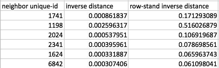
Figure 16: Inverse distance weights

As a result, the spatial lag computed with row-standardized inverse distance weights is similar in scale to the original variable (and similar to the spatial lags based on connectivity weights). This is illustrated by the results in Figure 15, under the heading IDRSND.

The fourth option is listed for completeness only, under the heading IDRSWD. In the implementation for connectivity weights, all observations end up with an equal weight. Specifically, this amounts to \(1 / (k_i + 1)\), where \(k_i\) is the number of neighbors for observation \(i\). In contrast, in the inverse distance case, each neighboring observation is scaled by a different weight, so that it is not clear what weight should be given to the diagonal element. In GeoDa, the diagonal element gets the value of 1, so that the spatial lag amounts to: \[[Wy]_i = y_i + \sum_j w_{ij} y_j.\] Again, this should only be used when there is a strong substantive motivation.

Spatially lagged variables from kernel weights

Spatially lagged variables can also be computed from kernel weights. However, in this instance, only one of the options with respect to row-standardization and diagonal weights makes sense. Since the kernel weights are the result of a specific kernel function, they should not be altered. Also, each kernel function results in a specific value for the diagonal element, which should not be changed either. As a result, the only viable option to create spatially lagged variables based on kernel weights is to have no row-standardization and have the diagonal elements included.

When the calculator spatial lag interface detects the selection of kernel weights, the options are greyed out, with the diagonal elements checked, as in Figure 17.⁴ The entry in the weight box, clev_sls_154_core_k6epadiag, refers to the Epanechnikov kernel weights computed for 6 nearest neighbors.

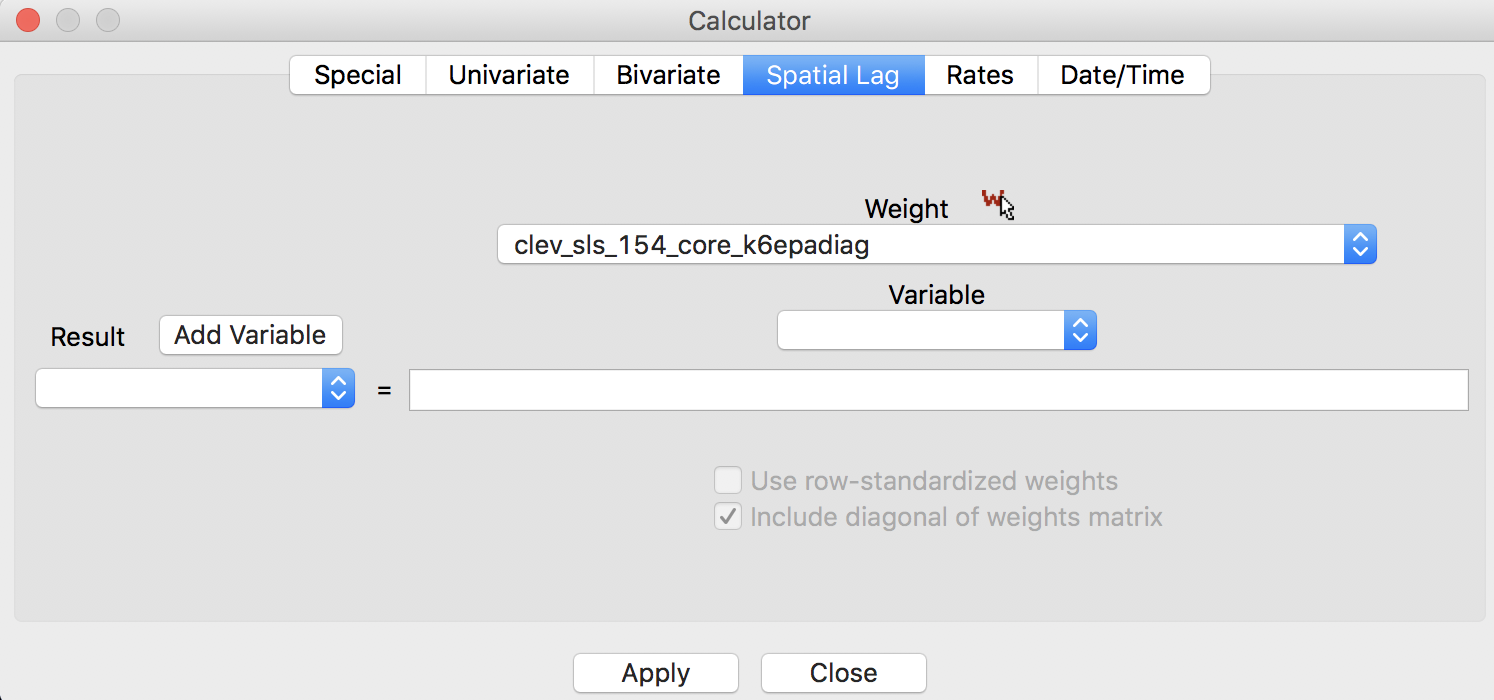
Figure 17: Kernel weights lag default options

The resulting spatially lagged variable is \[[Wy]_i = \sum_j K_{ij} y_j,\] where the sum includes the diagonal element of the kernel weight \(K_{ij}\). The results for the Epanechnikov weights (with 0.75 on the diagonal) are shown in Figure 18, under the heading EPALAG.

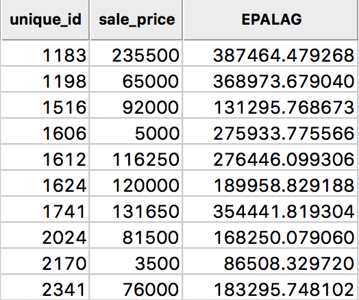
Figure 18: Epanechnikov kernel spatial lags for sales price in table

Kernel-based spatially lagged variables correspond to a form of local smoothing. They can be used in specialized regression specifications, such as geographically weighted regression (GWR).⁵

Principle

A spatial rate smoother is a special case of a nonparameteric rate estimator, based on the principle of locally weighted estimation (see, e.g., Waller and Gotway 2004, 89–90). Rather than applying a local average to the rate itself, as in an application of a spatial window average, the weighted average is applied separately to the numerator and denominator.

The spatially smoothed rate for a given location \(i\) is then given as: \[\pi_i = \frac{\sum_{j=1}^n w_{ij} O_j}{\sum_{j=1}^n w_{ij} P_j},\] where \(O_j\) is the event count in location \(j\), \(P_j\) is the population at risk, and \(w_{ij}\) are the spatial weights (typically with \(w_{ii} \neq 0\), i.e., including the diagonal).

Different smoothers are obtained for different spatial definitions of neighbors and/or different weights applied to those neighbors (e.g., contiguity weights, inverse distance weights, or kernel weights).⁶

An early example was the spatial rate smoother outlined in Kafadar (1996), based on the notion of a spatial moving average or window average (see also Kafadar 1997). The window average is not applied to the rate itself, but it is computed separately for the numerator and denominator. The simplest case boils down to applying the idea of a spatial window sum to the numerator and denominator (i.e., with binary spatial weights in both, and including the diagonal term): \[ \pi_i = \frac{O_i + \sum_{j=1}^{J_i} O_j}{P_i + \sum_{j=1}^{J_i} P_j},\] where \(J_i\) is a reference set (neighbors) for observation \(i\). In practice, this is achieved by using binary spatial weights for both numerator and denominator, and including the diagonal in both terms, as in the expression above.

A map of spatially smoothed rates tends to emphasize broad spatial trends and is useful for identifying general features of the data. However, it is not useful for the analysis of spatial autocorrelation, since the smoothed rates are autocorrelated by construction. It is also not very useful for identifying outlying observations, since the values portrayed are really regional averages and not specific to an individual location. By construction, the values shown for individual locations are determined by both the events and the population sizes of adjoining spatial units, which can lead to misleading impressions. Often, inverse distance weights are applied to both the numerator and denominator, e.g., as in the early discussion by Kafadar (1996).

Preliminaries

We return to the rate smoothing examples using the Ohio county lung cancer data. Therefore, we need to close the current project and load the ohlung data set.

Next, we need to create the spatial weights files we will use if we don’t have them already stored in a project file. In order to make sure that some smoothing will occur, we take a fairly wide definition of neighbors.⁷ Specifically, we will create a second order queen contiguity, inclusive of first order neighbors, inverse distance weights based on knn = 10 nearest neighbor weights, and Epanechnikov kernel weights, using the same 10 nearest neighbors and with the kernel applied to the diagonal (its value will be 0.75).

We proceed in the usual manner and use FIPSNO as the ID variable. The creation of the queen contiguity weights is straightforward (we name the file ohlung_q2inc). We postpone the creation of the inverse distance and kernel weights until the next section.

In addition to the spatial weights, we also need an example for crude rates. If not already saved in the data set, we compute the crude rate for lung cancer among white females in 68.

Using the Rates tab in the calculator, we first add a new variable, e.g., LRATE, then compute the crude rate with LFW68 as the Event Variable and POPFW68 as the Base Variable. In order to present the results on a more intuitive scale, we also multiply LRATE by 10,000, using the Bivariate tab with the Multiply function (the result gives the number of lung cancer cases per 10,000 white females). A standard deviational map for the rates, shown in Figure 19, illustrates the familiar pattern from the Chapter on mapping rates.

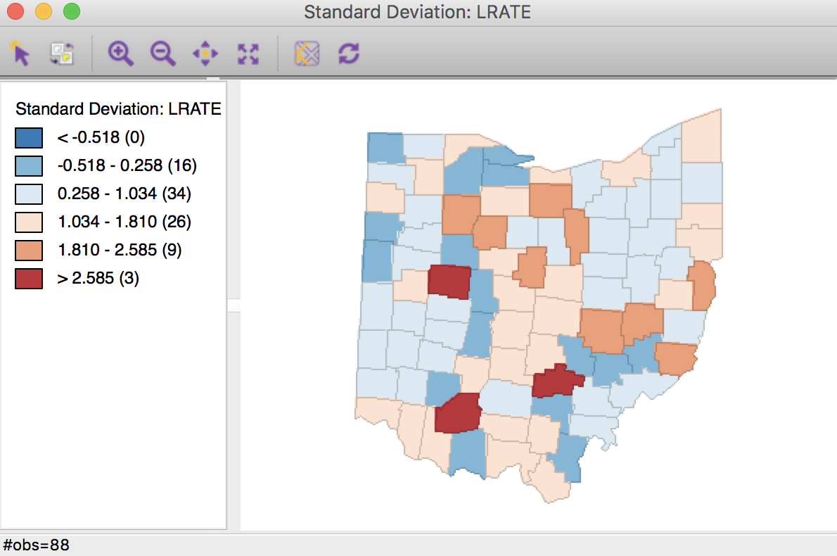
Figure 19: Standard deviational map for crude rates

Digression - rescaling coordinates

As pointed out in the discussion of inverse distance weights, the resulting values for the weights depend critically on the scale in which the (centroid) coordinates are expressed. In the example for Ohio counties, the unit of measurement is feet, which results in very large values for the coordinates. For example, if we use Shape Centers > Add Centroids to Table from the map, we can inspect the actual values under COORD_X and COORD_Y in the table shown in Figure 20.

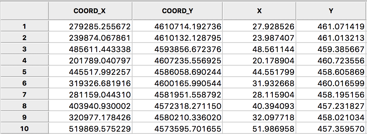
Figure 20: Rescaled centroid coordinates for Ohio counties

The magnitudes are in the hundreds of thousands and even in the millions (for the y-coordinate). As a result, the inter-point distances will be very large, and the corresponding inverse distance measures will be very small. For example, in the left-hand panel of Figure 21, we see the inverse distance weights for the 10 nearest neighbors of the county with FIPSNO 39095 (Lucas county, OH). The weights are all smaller than 0.0001. This will result in spatially lagged values that are very close to zero, and will not provide a meaningful averaging.

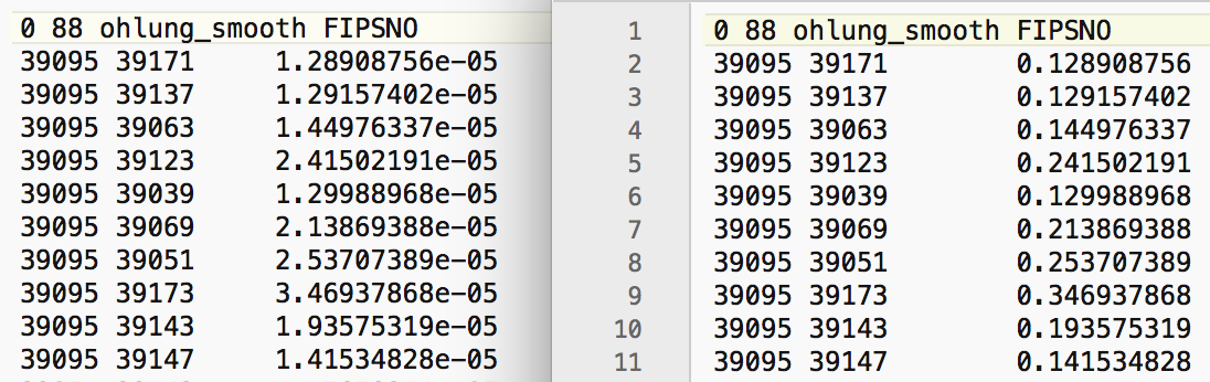
Figure 21: Inverse distance weights for Ohio counties

In order to fix this problem, we need to rescale the original coordinates. Using the calculator tool in the table, we create two new variables, X and Y, that are the original coordinates divided by 10000 (as above in the rescaling of the crude rates, use the Bivariate tab with the Divide function). The results are shown in the X and Y columns of Figure 20, and now represent units of 10000 feet.

As we have seen, we can use any two variables as coordinates for the distance weights. By selecting X and Y, we create a set of inverse distance weights to the 10 nearest neighors (as ohlung_k10invd). The corresponding values for the weights are shown in the right-hand panel of Figure 21. Compared to the original set, these are much more reasonable (all are larger than 0.1).

In addition to the queen contiguity and inverse distance weights, we also create Epanechnikov kernel weights (with the kernel applied to the diagonal) using an adaptive kernel for 10 nearest neighbors (i.e., with the same range as the inverse distance weights). We again use the X and Y coordinates to compute the distances. This yields the weights ohlung_epa.

At this point, we should have the three spatial weights listed in the weights manager panel, as in Figure 22. In our example, we show the properties of the second order contiguity weights. The number of neighbors ranges from 7 to 22, with an average of 14.64, which will yield some degree of smoothing. Of course, for the inverse distance and kernel weights, the number of neighbors is 10 for all counties.

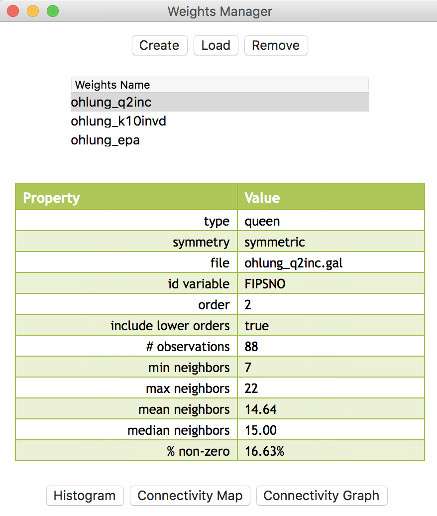
Figure 22: Weights manager for Ohio counties

We are now ready to proceed with the analysis.

Simple window average of rates

First, we illustrate how not to proceed, but use this as a reference. We compute the lag variable as a window average, using the settings in the calculator. We select the Spatial Lag tab shown in Figure 10, with both the Use row-standardized weights and the Include diagonal of weights matrix boxes checked in the interface. We specify ohlung_q2inc as the spatial weight and LRATE as the variable. The window average is contained in the new variable W_LRATE. The calculator interface should be as in Figure 23.

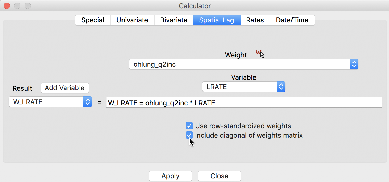
Figure 23: Spatial window average of crude rates

The corresponding standard deviational map is given in Figure 24.

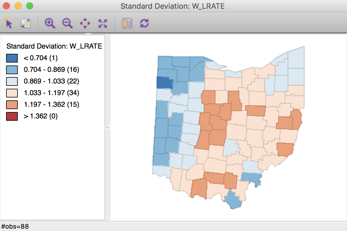
Figure 24: Crude rate spatial window average

Characteristic of the spatial averaging, several larger groupings of similarly classified observations appear. The pattern is quite different from that displayed for the crude rate in Figure 19. For example, the upper outliers have disappeared, and there is now one new lower outlier.

Spatially smoothed rates

As mentioned, applying the spatial averaging directly to the crude rates is not the proper way to operate. This approach ignores the differences between the populations of the different counties and the associated variance instability of the rates. The Spatial Rate smoothing option is the correct alternative, which applies the smoothing separately to the observations as they enter into the numerator and the denominator of the rate calculation.

We invoke this calculation either from the menu, as Map > Rates-Calculated Map > Spatial Rate, or by right-clicking on the current map and selecting Rates > Spatial Rate, as shown in Figure 25.

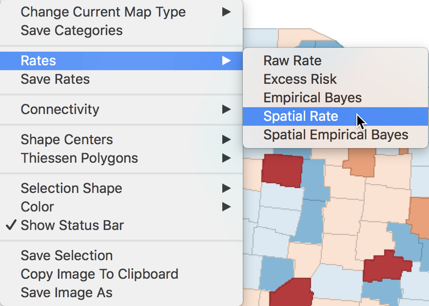
Figure 25: Spatial rate option

The dialog that appears, shown in Figure 26, is the usual interface for rate calculation. It requires the selection of the Event Variable (LFW68), the Base Variable (POPFW68), the Map Theme (Standard Deviation Map), and a specification for the spatial weights (ohlung_q2inc).⁸

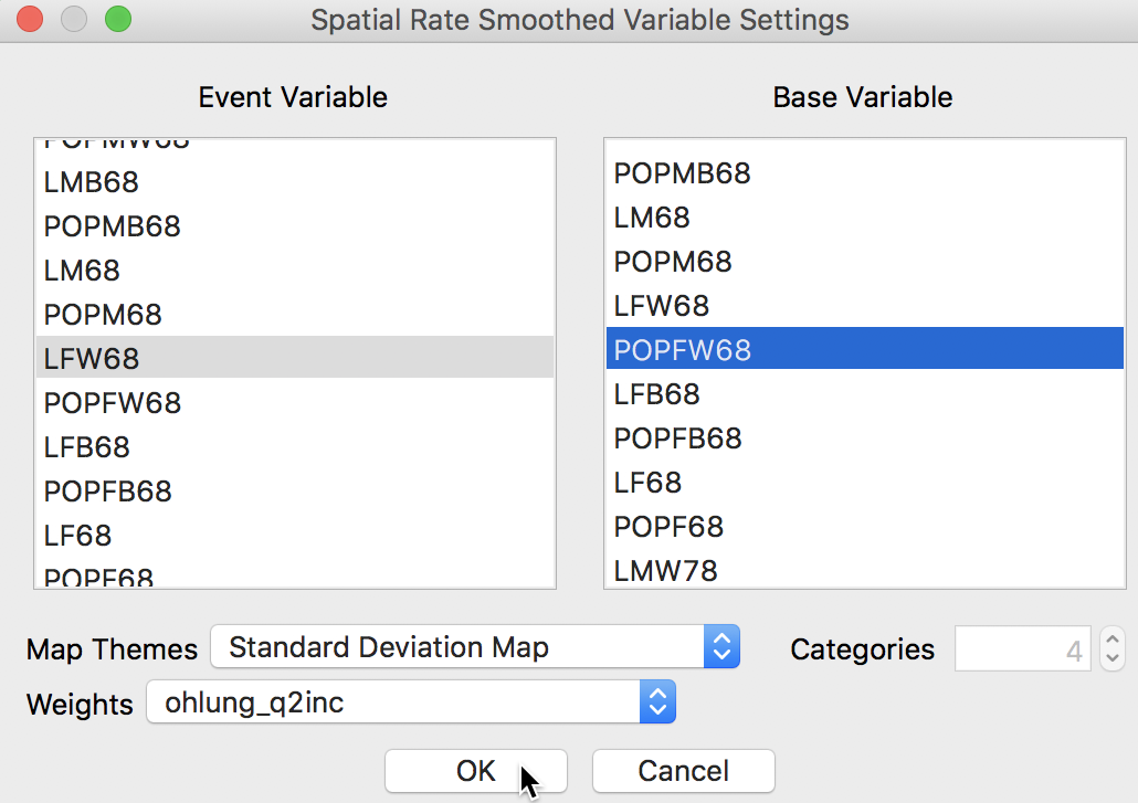
Figure 26: Spatial rate dialog

Clicking OK brings up a standard deviation map with the smoothed rates, shown in Figure 27.

In order to make the category ranges meaningful, we use a legend option to give the results in scientific notation (right click on the legend pane and select Use Scientific Notation). Again, we observe the larger groupings of observations, but now several outliers remain, although not in the same locations as for the crude rate.

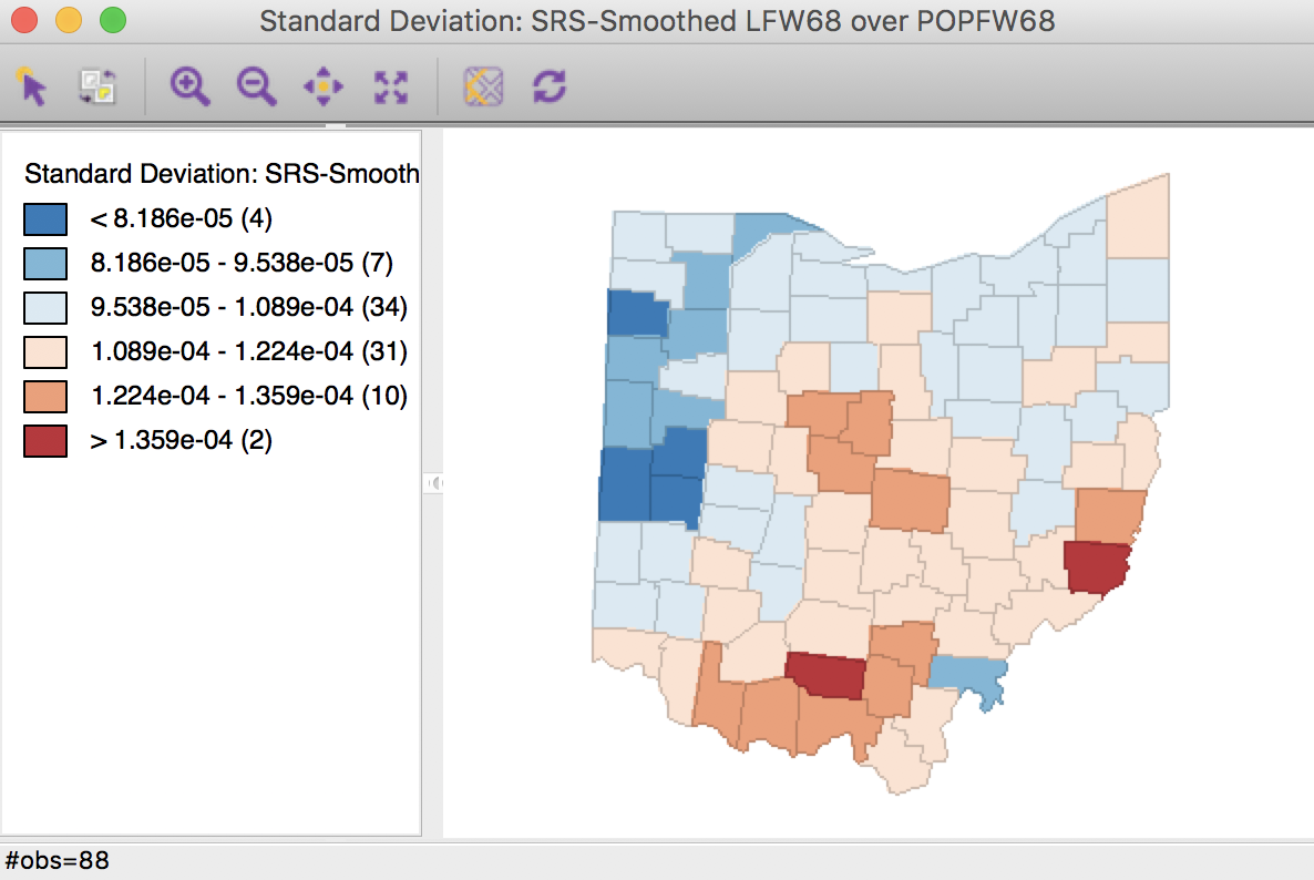
Figure 27: Spatial rate smoothed map

We add the smoothed rates to the data table by means of the Save Rates option (keeping the default variable name of R_SPAT_R). As we did above for LRATE, we multiply the ratio by 10,000 in the calculator to make the results easier to interpret. The three sets of rates are shown in the table in Figure 28 for the first ten counties.

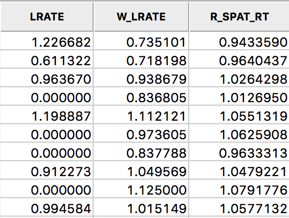
Figure 28: Comparison of smoothed rates in table

A more quantified comparison is obtained from a scatter plot of W_LRATE against R_SPAT_RT. As is clear from Figure 29, the values are far from the same. In fact, the R² of the linear fit is only 0.60.

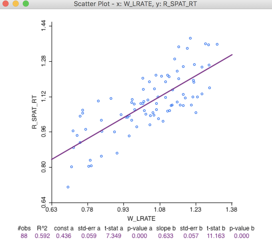
Figure 29: Comparison of spatial rates

Spatially smoothed rates in the table

The spatial rate smoothing option is only implemented for contiguity weights, i.e., an unweighted average is calculated for both the numerator and denominator. Of course, we can also carry this out explicitly, by creating separate spatially lagged variables for the counts of events and for the populations at risk (using the spatial window average operation covered earlier), followed by their ratio (and possibly scaling by a factor such as 10000).

If inverse distance or kernel weights are specified in the spatial rate variable setting dialog (Figure 26), the values for the weights are ignored, and only the connectivity information is taken into account to compute the averages. As an alternative, we can carry out the explicit spatial lag calculation for the numerator and denominator, which will use the actual weights in the computation. This is can be accomplished with the Calculator option in the table.

We first proceed with the inverse distance weights (ohlung_k10invd). We proceed in the calculator in turn for the numerator and denominator. We add a new variable for each, and then compute the spatial window sum using the inverse distance weights applied to LFW68 and POPFW68. The options should be set to not row-standardize the weights and to include the diagonal (the option should be checked as in Figure 12). We next create a new variable, IDRATE, as the ratio of the numerator over the denominator, and rescale by multiplying with 10000. The corresponding standard devational map is shown in Figure 30.

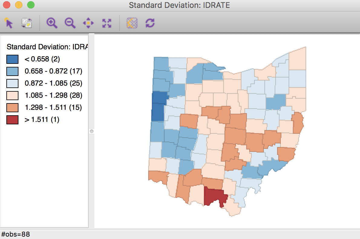
Figure 30: Inverse distance spatial rate smoothed map

We can also apply the same technique to kernel weights, e.g. using ohlung_epa. Following the same steps as for the inverse distance weights, with the same settings in the dialog will yield rates that are smoothed using the weights determined by the kernel function. This yields the standard deviational map shown in Figure 31.

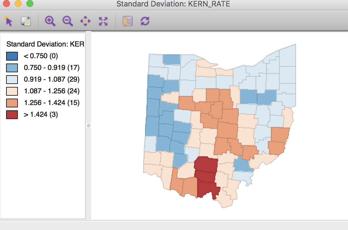
Figure 31: Kernel weights spatial rate smoothed map

It is important to keep in mind that both the inverse distance and kernel weights spatially smoothed rates are based on a particular trade-off between the value at the location and its neighbors. This trade-off depends critically on the distance metric used in the calculations (or, on the scale in which the coordinates are expressed). There is no right answer, and a thorough sensitivity analysis is advised.

For example, we can observe that the three spatially smoothed maps in Figures 27, 30, and 31 point to some elevated rates in the south of the state, but the extent of the respective regions and the counties on which they are centered differ slightly. Also, the general regional patterns are roughly the same, but there are important differences in terms of the specific counties affected.

In the table shown in Figure 32, we summarize all the rates computed in this section: LRATE is the crude rate, W_LRATE it its queen contiguity based spatial lag, R_SPAT_RT is the spatially smoothed rate saved from the calculation, IDRATE is the rate based on inverse distance weights, KERN_RATE the kernel-smoothed rate, and S_LRATE is the spatially smoothed rate computed in the table as an explicit ratio between numerator and denominator (it is identical to the result from the direct rate calculation in R_SPAT_RT).

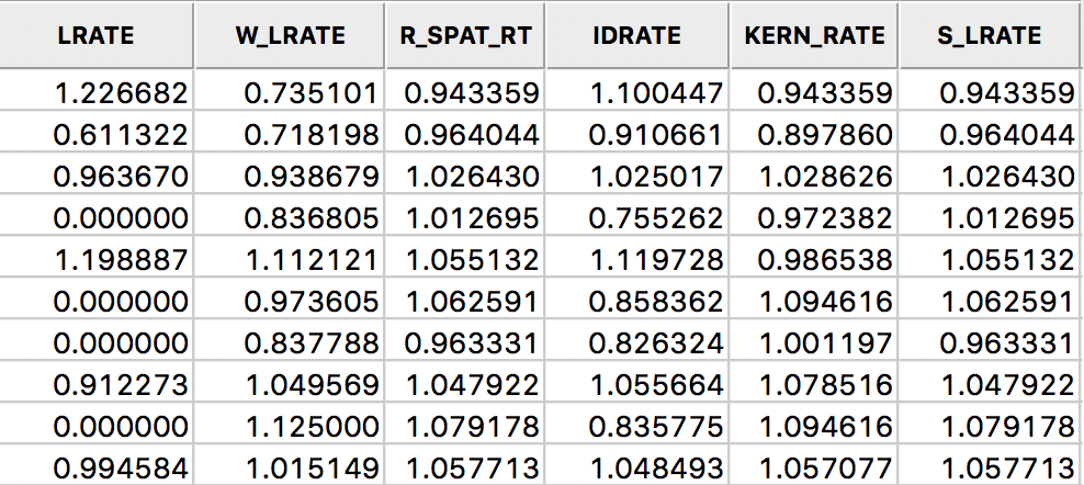
Figure 32: All spatially smoothed rates in the table

Principle

The second option for spatial rate smoothing is Spatial Empirical Bayes. This operates in the same way as the standard Empirical Bayes smoother (covered in the rate mapping Chapter), except that the reference rate is computed for a spatial window for each individual observation, rather than taking the same overall reference rate for all. This only works well for larger data sets, when the window (as defined by the spatial weights) is large enough to allow for effective smoothing.

Similar to the standard EB principle, a reference rate (or prior) is computed. However, here, this rate is estimated from the spatial window surrounding a given observation, consisting of the observation and its neighbors. The neighbors are defined by the non-zero elements in the row of the spatial weight matrix (i.e., the spatial weights are treated as binary).

Formally, the reference mean for location \(i\) is then: \[\mu_i = \frac{\sum_j w_{ij} O_j}{\sum_j w_{ij} P_j},\] with \(w_{ij}\) as binary spatial weights, and \(w_{ii} = 1\).

The local estimate of the prior variance follows the same logic as for EB, but replacing the population and rates by their local counterparts: \[\sigma^2_i = \frac{\sum_j w_{ij}[ P_j (r_i - \mu_i)^2] }{\sum_j w_{ij} P_j} - \frac{\mu_i}{\sum_j w_{ij} P_i / (k_i +1)}.\] Note that the average population in the second term pertains to all locations within the window, therefore, this is divided by \(k_i + 1\) (with \(k_i\) as the number of neighbors of \(i\)). As in the case of the standard EB rate, it is quite possible (and quite common) to obtain a negative estimate for the local variance, in which case it is set to zero.

The spatial EB smoothed rate is computed as a weighted average of the crude rate and the prior, in the same manner as for the standard EB rate (see the discussion in the Chapter on mapping rates, as well as Anselin, Lozano-Gracia, and Koschinky 2006, for technical details).

Spatial EB rate smoother

The spatial Empirical Bayes rate smoother is invoked from the menu as Map > Rates-Calculated Map > Spatial Empirical Bayes, or from the option menu in any map, as Rates > Spatial Empirical Bayes. The latter is illustrated in Figure 33.

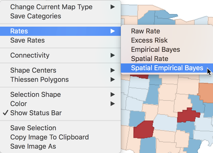
Figure 33: Spatial Empirical Bayes option

The variable settings dialog is identical to that for the spatial rate smoother, as shown in Figure 26. We can use the exact same settings, with the second order queen contiguity defining the range of the window for each observation.

Using these settings, a standard deviational map of the smoothed rates is as in Figure 34.

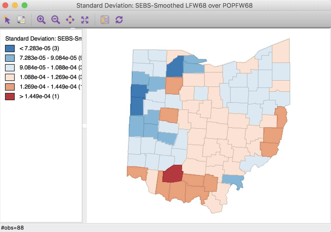
Figure 34: Spatial EB rate using second order queen contiguity

Selecting the inverse distance weights results in the map shown in Figure 35. Note that the actual inverse distance weights are ignored, but only used to identify the 10 nearest neighbors for each location. This defines the spatial window for which the local priors are computed.

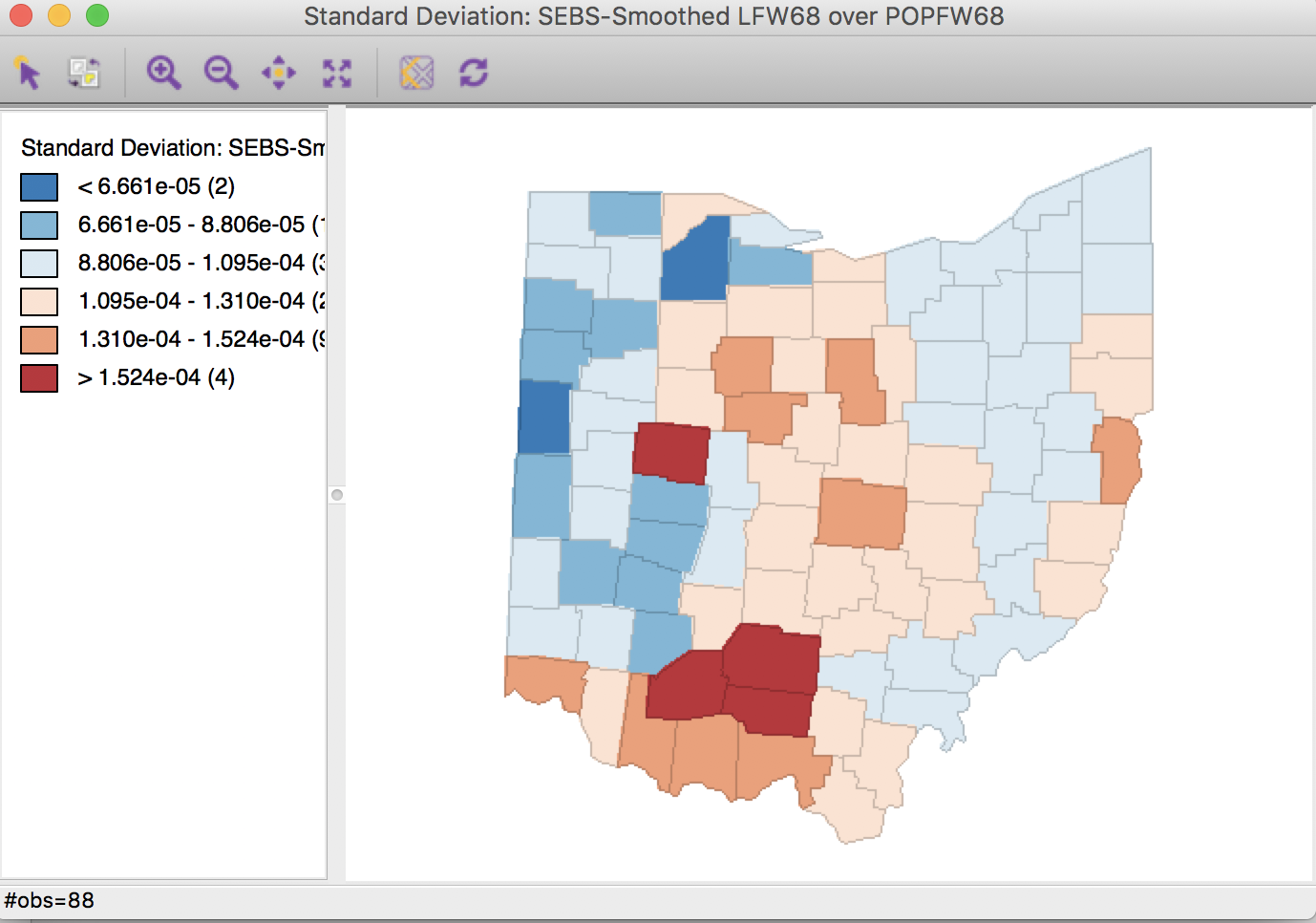
Figure 35: Spatial EB rate using k = 10 nearest neighbors

As for the spatial rate smoothing approaches, a careful sensitivity analysis is in order. The results depend considerably on the range used for the reference rate. The larger the range, the more the smoothed rates will be similar to the global EB rate. For a narrow range, the estimate of the local variance will often result in a zero imputed value, which makes the EB approach less meaningful.

References

Anselin, Luc, Nancy Lozano-Gracia, and Julia Koschinky. 2006. “Rate Transformations and Smoothing.” Technical Report. Urbana, IL: Spatial Analysis Laboratory, Department of Geography, University of Illinois.
Fotheringham, A. Stewart, Chris Brunsdon, and Martin Charlton. 2002. Geographically Weighted Regression. Chichester: John Wiley.
Kafadar, Karen. 1996. “Smoothing Geographical Data, Particularly Rates of Disease.” Statistics in Medicine 15:2539–60.
———. 1997. “Geographic Trends in Prostate Cancer Mortality: An Application of Spatial Smoothers and the Need for Adjustment.” Annals of Epidemiology 7:35–45.
Waller, Lance A., and Carol A. Gotway. 2004. Applied Spatial Statistics for Public Health Data. Hoboken, NJ: John Wiley.
-
University of Chicago, Center for Spatial Data Science – anselin@uchicago.edu↩
The GWT file also includes the respective distances, but these are ignored in the spatial lag operations.↩
After re-arranging the columns in the table, the variable name listed under Variable in the interface may have changed. In our example, it should be sale_price.↩
While this option is not available as a selection, it is set by default. Displaying the check mark in the interface makes clear which options are being used.↩
GWR is not implemented in GeoDa. For further details on the use of kernel-based spatially lagged variables in GWR, see, e.g., Fotheringham, Brunsdon, and Charlton (2002).↩
For further details, see Anselin, Lozano-Gracia, and Koschinky (2006), Section 5.2.↩
If the spatial window over which the average is computed is not sufficiently wide, such as with first order contiguity weights, very little smoothing occurs, and the results may be somewhat erratic.↩
Alternatively, we can compute the spatial rates in the calculator, using the Rates tab. Note that the weights information in inverse distance weights and kernel weights is ignored in this operation, only the connectivity is used to compute the spatial averages.↩