Global Spatial Autocorrelation (2)
Bivariate, Differential and EB Rate Moran Scatter Plot
Luc Anselin1
03/06/2019 (latest update)
Introduction
In this Chapter, we consider some extensions to the visualization of spatial autocorrelation by means of the Moran scatter plot. Specifically, we extend the association between a variable and its spatial lag to the context where the variable and the lag pertain to two different variables, in the form of a bivariate Moran scatter plot. We focus on this specifically in the context of relating a variable to its neighbors in a different time period. We also consider a refinement of this concept that applies the notion of a Moran scatter plot to the first difference (or any difference) of time-enabled variables, as the differential Moran scatter plot. We close with an adjustment of Moran’s I designed to deal with the variance instability of rates or proportions, the EBI Moran scatter plot.
We will again use the U.S. County Homicides sample data set that comes pre-installed with GeoDa. It contains values for homicides and several socio-economic determinants for the 3085 counties in the continental United States.
Objectives
-
Visualize bivariate spatial correlation
-
Assess different aspects of bivariate spatial correlation
-
Visualize bivariate spatial correlation among time-differenced values
-
Correct Moran’s I for the variance instability in rates
GeoDa functions covered
- Space > Bivariate Moran’s I
- variable selection
- permutation inference
- saving the spatial lag
- Moran scatter plot options
- Space > Differential Moran’s I
- saving the first differences and spatial lag
- Space > Moran’s I with EB Rate
- saving the rate
Getting Started
Before exploring the bivariate extensions, we turn a few of the variables in the natregimes data set into time-enabled variables. Specifically, using the techniques illustrated earlier, we group the homicide rates hr60 through hr90 into hr, the homicide counts hc60 to hc90 into hc, and the population counts po60 through po90 into po.
In addition to the grouped variables, we also need to create at least one spatial weights matrix, e.g., natregimes_q for first order queen contiguity.
After saving all this information into a project file, we clear the current project and load the new project file into the Connect to Data Sources dialog. This brings up the familiar green themeless U.S. counties map.
Bivariate Spatial Correlation - A Word of Caution
The concept of bivariate spatial correlation is complex and often misinterpreted. It is typically considered to be the correlation between one variable and the spatial lag of another variable, as originally implemented in the precursor of GeoDa (e.g., as described in Anselin, Syabri, and Smirnov 2002). However, this does not take into account the inherent correlation between the two variables. More precisely, the bivariate spatial correlation is between \(x_i\) and \(\sum_j w_{ij} y_j\), but does not take into account the correlation between \(x_i\) and \(y_i\), i.e., between the two variables at the same location.
As a result, this statistic is often interpreted incorrectly, as it may overestimate the spatial aspect of the correlation that instead may be due mostly to the in-place correlation. Lee (2001) provides an alternative that considers a separation between the correlative aspect and the spatial aspect, but we will not pursue that here.
Below, we provide a more in-depth assessment of the different aspects of bivariate spatial and non-spatial association, but first we turn to the original concept of a bivariate Moran scatter plot.
Bivariate Moran Scatter Plot
Concept
In its initial conceptualization, as mentioned above, a bivariate Moran scatter plot extends the idea of a Moran scatter plot with a variable on the x-axis and its spatial lag on a y-axis to a bivariate context. The fundamental difference is that in the bivariate case the spatial lag pertains to a different variable. In essence, this notion of bivariate spatial correlation measures the degree to which the value for a given variable at a location is correlated with its neighbors for a different variable.
As in the univariate Moran scatter plot, the interest is in the slope of the linear fit. This yields a Moran’s I-like statistic as: \[I_B = \frac{\sum_i (\sum_j w_{ij} y_j \times x_i)}{ \sum_i x_i^2},\] or, the slope of a regression of \(Wy\) on \(x\).
As before, all variables are expressed in standardized form, such that their means are zero and their variance one. In addition, the spatial weights are row-standardized.
Note that, unlike in the univariate autocorrelation case, the regression of \(x\) on \(Wy\) also yields an unbiased estimate of the slope, providing an alternative perspective on bivariate spatial correlation (see below for further discussion).2
A special case of bivariate spatial autocorrelation is when the variable is measured at two points in time, say \(z_{i,t}\) and \(z_{i,t-1}\). The statistic then pertains to the extent to which the value observed at a location at a given time, is correlated with its value at neighboring locations at a different point in time.
The natural interpretation of this concept is to relate \(z_{i,t}\) to \(\sum_j w_{ij} z_{j,t-1}\), i.e., the correlation between a value at \(t\) and its neighbors in a previous time period: \[I_T = \frac{\sum_i (\sum_j w_{ij} z_{j,t-1} \times z_{i,t})}{ \sum_i z_{i,t}^2},\] i.e., the effect of neighbors in \(t-1\) on the present value.
Alternatively, and maybe less intuitively, one can relate the value at a previous time period \(z_{t-1}\) to its neighbors in the future, \(\sum_j w_{ij} z_t\), as: \[I_T = \frac{\sum_i (\sum_j w_{ij} z_{j,t} \times z_{i,t-1})}{ \sum_i z_{i,t-1}^2},\] i.e., the effect of a location at \(t-1\) on its neighbors in the future.
While formally correct, this may not be a proper interpretation of the dynamics involved. In fact, the notion of spatial correlation pertains to the effect of neighbors on a central location, not the other way around. While the Moran scatter plot seems to reverse this logic, this is purely a formalism, without any consequences in the univariate case. However, when relating the slope in the scatter plot to the dynamics of a process, this should be interpreted with caution.
A possible source of confusion is that the proper regression specification for a dynamic process would be as: \[z_{i,t} = \beta_1 \sum_j w_{ij} z_{j,t-1} + u_i,\] with \(u_i\) as the usual error term, and not as: \[z_{i,t-1} = \beta_2 \sum_j w_{ij} z_{j,t} + u_i,\] which would have the future predicting the past. This contrasts with the linear regression specification used (purely formally) to estimate the bivariate Moran’s I, for example: \[\sum_j w_{ij} z_{j,t-1} = \beta_3 z_{i,t} + u_i.\]
In terms of the interpretation of a dynamic process, only \(\beta_1\) has intuitive appeal. However, in terms of measuring the degree of spatial correlation between past neighbors and a current value, as measured by a Moran’s I coefficient, \(\beta_3\) is the correct interpretation.
As mentioned earlier, a fundamental difference with the univariate case is that the spatially lagged variable is no longer endogenous, so both specifications can be estimated by means of ordinary least squares.
In the univariate case, only the specification with the spatially lagged variable on the left hand side yields a valid estimate. As a result, for the univariate Moran’s I, there is no ambiguity about which variables should be on the x-axis and y-axis.
Inference is again based on a permutation approach, but with an important difference. Since the interest focuses on the bivariate spatial association, the values for \(x\) are fixed at their locations, and only the values for \(y\) are randomly permuted. In the usual manner, this yields a reference distribution for the statistic under the null hypothesis that the spatial arrangement of the \(y\) values is random. As mentioned, it is important to keep in mind that since the focus is on the correlation between the \(x\) value at \(i\) and the \(y\) values at the neighboring locations, the correlation between \(x\) and \(y\) at location \(i\) is ignored.
Creating a bivariate Moran scatter plot
The Bivariate Moran’s I is invoked from the menu or from the drop-down list provided by selecting the Moran Scatter Plot icon on the toolbar, shown in Figure 1.
Figure 1: Bivariate Moran scatter plot icon
The next dialog brings up the variable specification. In our example, we will illustrate the most useful way to employ bivariate spatial correlation, i.e., its application to assess the correlation between a variable and its neighbors at a different time period. Ignoring the in-situ temporal correlation, such a measure gives insight into the extent to which neighboring locations in a previous time period are correlated with the value at a location at a future time period. In other words, this gives some indication of space-time correlation (but also see below for a more refined analysis).
To illustrate this functionality, we select as the x-axis variable, the homicide rate in 1990 – hr (90) –, and as the y-axis its value in 1980 – hr (80) –, which will be the spatial lag. The dialog is the familiar one for time-enabled variables, with the Time drop down list allowing variables to be selected for different time periods, and the spatial weights specified in the Weights list. In our example, shown in Figure 2, the spatial weights are the queen contiguity weights, natregimes_q.
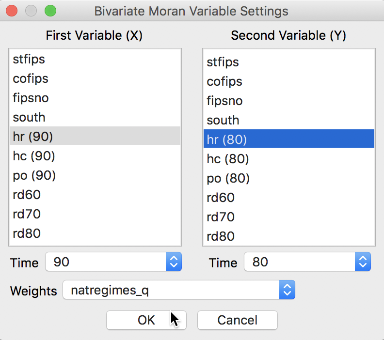
Figure 2: Bivariate Moran scatter variable selection
The bivariate Moran scatter plot shows a scatter plot with spatial lag of hr (80) (\(Wy\)) on the y-axis and hr (90) (\(x\)) on the x-axis. The slope of the linear fit is the bivariate Moran’s I (as defined above). In our example, this is about 0.360, as illustrated in Figure 3.
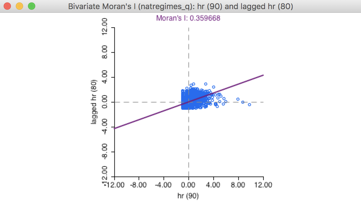
Figure 3: Bivariate Moran scatter plot
All the same options as for the univariate Moran scatter plot apply here as well. For example, a permutation inference would indicated a high significance of the association, with a pseudo p-value of 0.001 (for 999 permutations).3 Also, the standardized value of the x variable and the spatial lag of the y-variable (applied to its standardized value) can be saved to the table, in the same way as for the univariate Moran scatter plot.
A closer look at bivariate spatial correlation
In contrast to the univariate Moran scatter plot, where the interpretation of the linear fit is unequivocably Moran’s I, there is no such clarity in the bivariate case. In addition to the interpretation offered above, which is a traditional Moran’s I-like coefficient, there are at least four additional perspectives that are relevant. We consider each in turn.
Serial (temporal) correlation
First, we need to consider the bivariate correlation between the homicide rate in the two time periods, i.e., hr (90) and hr (80). To implement this, we create four new variables. First, we standardize the homicide rates for each of the years, say as hr80st and hr90st. Next, we compute the spatial lags for these variables using the queen contiguity weights, say whr80st and whr90st.4
The relation between hr90st and hr80st (or, in general, between a variable \(y_{i,t}\) and its time lag \(y_{i,t-1}\)) yields a highly significant slope of 0.553, as shown in the standard scatter plot graph in Figure 4. This suggests a very strong temporal correlation of this variable over time.
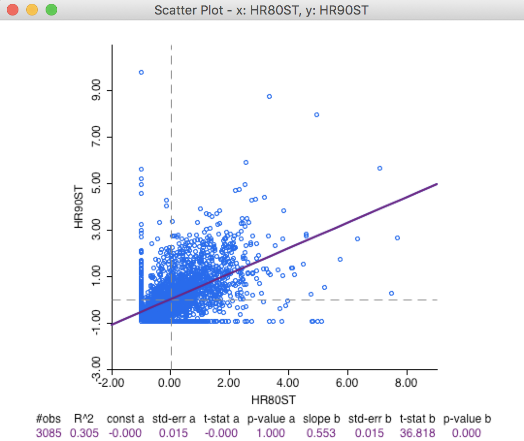
Figure 4: Scatter plot hr90 on hr80
Serial (temporal) correlation between spatial lags
Closely related to this temporal correlation is the linear relation between the spatial lag of the crime rates between the two time periods (i.e., a regression of the variable \(\sum_j w_{ij} y_{j,t}\) on \(\sum_j w_{ij} y_{j,t-1}\)). In some sense, if there is a strong temporal correlation between the variable in-situ, then it is likely that there is also a strong temporal correlation between their neighbors (in the form of their spatial lags). Again, the standard scatter plot yields a strongly significant positive slope of 0.801, even higher than for the variable in-situ, as listed in Figure 5.
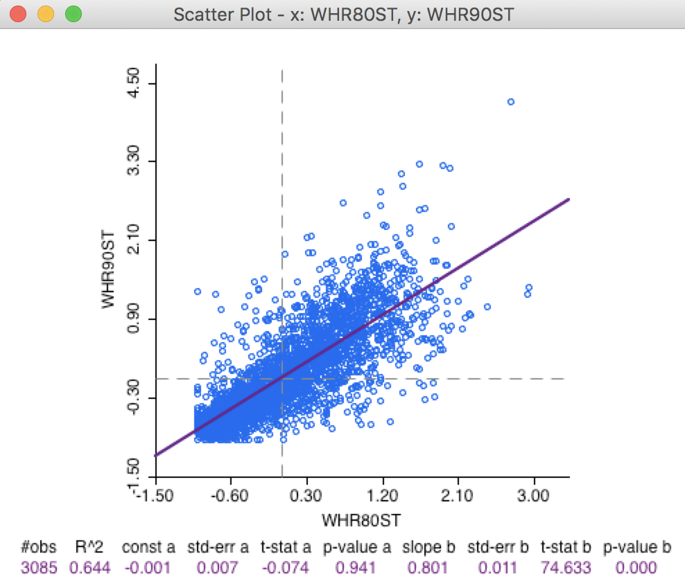
Figure 5: Scatter plot W_hr90 on W_hr80
Space-time regression
Thirdly, as mentioned earlier, there is no issue with regressing the value of hr90st on the spatial lag in 1980 (whr80st). Unlike what is the case in the pure cross-sectional situation, where the spatial lag is endogenous, the spatial lag in a different time period is exogenous (in the absence of temporal correlation).
The implication of this is that the ordinary regression estimate of the slope coefficient of hr90st on whr80st is unbiased. In the standard spatial scatter plot, this yields a slope of 0.746, again highly significant, as shown in Figure 6.
The specification with the value of a variable at time \(t\) regressed on the value of its neighbors at time \(t - 1\) (formally, a regression of \(y_{i,t}\) on \(\sum_j w_{ij} y_{j,t-1}\)) is the most natural formulation of a space-time regression, expressing how the values at neighboring locations at the previous time period diffuse to the location at the next time period.
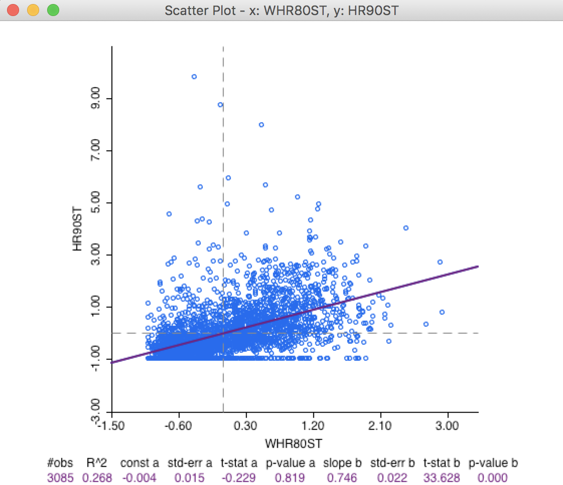
Figure 6: Scatter plot hr90 on W_hr80
Serial and space-time regression
Finally, we can include both in-situ correlation and space-time correlation in a regression specification of \(y_{i,t}\) (i.e., hr90st) on both \(x_{i,t-1}\) (i.e., hr80st) and \(\sum_j w_{ij}x_{j,t-1}\) (i.e., whr80st). In the absence of temporal error autocorrelation, standard ordinary least squares regression will yield unbiased estimates of the coefficients.
Using the regression functionality of GeoDa (not further considered here), this yields the result shown in Figure 7.
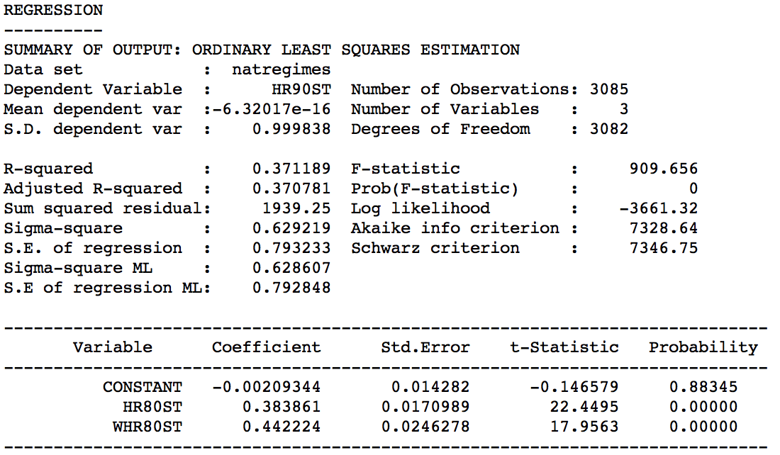
Figure 7: Bivariate lag decomposition regression
Correcting for both the in-situ correlation and the space-time correlation simultaneously considerably lowers the regression coefficients. In the regression, both effects are highly significant, with a coefficient of 0.384 for the in-situ effect, and 0.442 for the space-time effect.
Needless to say, focusing the analysis solely on the bivariate Moran scatter plot provides only a limited perspective on the complexity of space-time (or, in general, bivariate) spatial and space-time associations.
Differential Moran Scatter Plot
Concept
An alternative to the bivariate spatial correlation between a variable at one point in time and its neighbors at a previous (or, in general, any different) point in time is to control for the locational fixed effects by diffencing the variable. More precisely, we apply the computation of the spatial autocorrelation statistic to the variable \(y_{i,t} - y_{i,t-1}\).
This takes care of any temporal correlation that may be the result of a fixed effect (i.e. a set of variables determining the value of \(y_i\) that remain unchanged over time). Specifically, if \(\mu_i\) were a fixed effect associated with location \(i\), we could express the value at each location for time \(t\) as the sum of some intrinsic value and the fixed effect, as \(y_{i,t} = y*_{i,t} + \mu_i\), where \(\mu_i\) is unchanged over time (hence, fixed). The presence of \(\mu_i\) induces a temporal correlation between \(y_{i,t}\) and \(y_{i,t-1}\), above and beyond the correlation between \(y*_{i,t}\) and \(y*_{i,t-1}\). Taking the first difference eliminates the fixed effect and ensures that any remaining correlation is solely due to \(y*\).
A differential Moran’s I is then the slope in a regression of the spatial lag of the difference, i.e., \(\sum_j w_{ij} (y_{j,t} - y_{j,t-1})\) on the difference \((y_{i,t} - y_{i,t-1})\). Note that in GeoDa, the slope computation is applied to the standardized value of the difference (i.e., the standardization of \(y_{i,t} - y_{i,t-1}\)), and not to the difference between the standardized values.
All the caveats and different interpretations that apply to the generic bivariate case are also relevant here.
Implementation
We start the differential Moran scatter plot in the by now familiar way, from the main menu as Space > Differential Moran’s I, or from the Moran scatter plot toolbar icon, as the third item in the drop down list, shown in Figure 8.
Note that this functionality is only available for data sets with grouped variables. If there are no grouped variables present, a warning message will be generated.
Figure 8: Differential Moran scatter plot icon
With grouped variables in the data set, selecting the option brings up the variable selection dialog. This contains four drop down lists, as illustrated in Figure 9.
The Select variable list contains only the grouped variables. In our example, this is hr, hc and po, as shown. The next two drop down lists allow the time periods to be chosen (these correspond to the time labels entered when creating the grouped variables). Finally, the list at the bottom allows for the selection of the spatial weights. In our example, we take hr between 90 and 80 with the natregimes_q spatial weights.
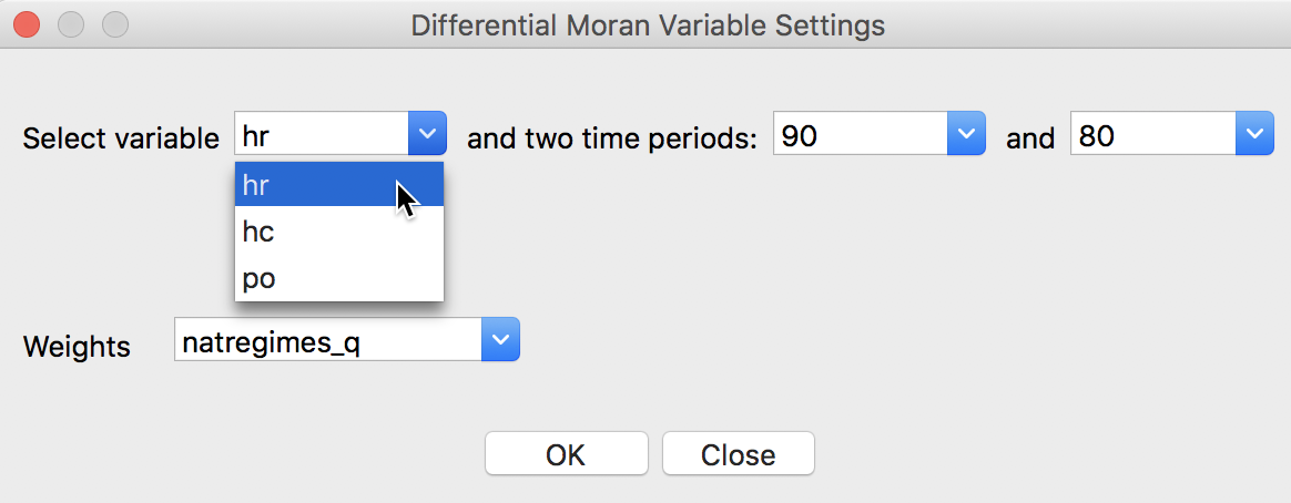
Figure 9: Differential Moran variable selection
The result is the familiar plot, shown in Figure 10. The slope is about 0.052, much smaller in magnitude than the bivariate space-time measures obtained so far. Of course, the same plot could have been obtained from the standard univariate Moran scatter plot, after first creating the first differences in the table calculator.
Even with this small value for Moran’s I, the statistic is highly significant. Permutation inference (not shown) with 999 replications yields a pseudo p-value of 0.001 and corresponding z-value of 5.03.5
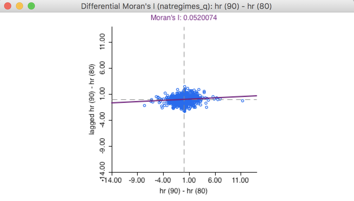
Figure 10: Differential Moran scatter plot
Options
All the standard Moran scatter plot options also apply to the differential plot.
For example, after activating the View > Regimes Regression option, we can investigate the difference between regionalized autocorrelation coefficients. In the same manner as we implemented for the standard Moran scatter plot, we can select a subset of observations, such as the counties in the south, and assess the effect on the autocorrelation coefficient.
In Figure 11, the Moran scatter plot on the left shows the value for the 1321 selected observations as 0.0658, with the value for the complement (unselected) as 0.0314, compared to the overall coefficient of 0.052. As before, this is purely illustrative and is not associated with a formal test for structural stability.
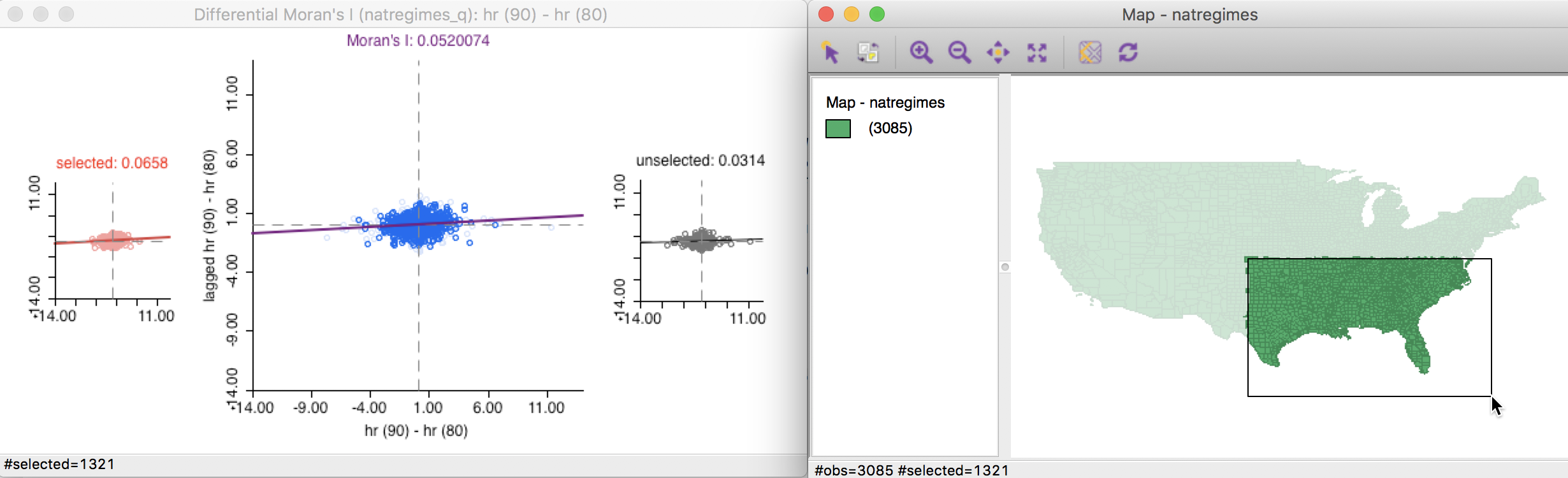
Figure 11: Brushing the differential Moran scatter plot
Finally, the option to Save Results works in a slightly different fashion from the standard case. In addition to the standardized value (of \(y_{i,t} - y_{i,t-1}\)) and its spatial lag, the actual first difference (in unstandardized form) can be saved to the table as well, when the Diff Values box is checked, as in Figure 12.
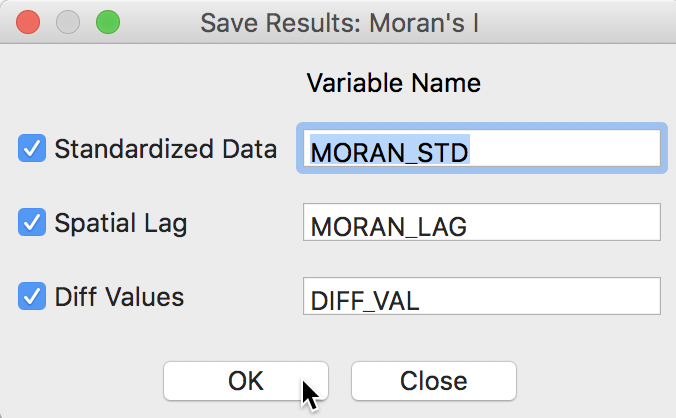
Figure 12: Saving the first difference and its spatial lag
Moran Scatter Plot for EB Rates
Concept
An Empirical Bayes (EB) standardization was suggested by Assunção and Reis (1999) as a means to correct Moran’s I spatial autocorrelation test statistic for varying population densities across observational units, when the variable of interest is a rate or proportion. This standardization borrows ideas from the Bayesian shrinkage estimator outlined in discussion of Empirical Bayes smoothing.
This approach is different from EB smoothing in that the spatial autocorrelation is not computed for a smoothed version of the original rate, but for a transformed standardized random variable. In other words, the crude rate is turned into a new variable that has a mean of zero and unit variance, thus avoiding problems with variance instability. The mean and variance used in the transformation are computed for each individual observation, thereby properly accounting for the instability in variance.
The technical aspects are given in detail in Assunção and Reis (1999) and in the review by Anselin, Lozano-Gracia, and Koschinky (2006), but we briefly touch upon some salient issues here. The point of departure is the crude rate, say \(r_i = O_i / P_i\), where \(O_i\) is the count of events at location \(i\) and \(P_i\) is the corresponding population at risk.
The rationale behind the Assuncao-Reis approach is to standardize each \(r_i\) as \[z_i = \frac{r_i - \beta}{\sqrt{\alpha + (\beta / P_i)}},\] using an estimated mean \(\beta\) and standard error \(\sqrt{\alpha + \beta / P_i}\). The parameters \(\alpha\) and \(\beta\) are related to the prior distribution for the risk, which we detailed in the Chapter on rate mapping.
In practice, the prior parameters are estimated by means of the so-called method of moments (e.g., Marshall 1991), yielding the following expressions: \[\beta = O / P,\] with \(O\) as the total event count (\(\sum_i O_i\)), and \(P\) as the total population count (\(\sum_i P_i\)), and \[\alpha = [\sum_i P_i ( r_i - \beta )^2 ] / P - \beta / ( P / n),\] with \(n\) as the total number of observations (in other words, \(P/n\) is the average population).
One problem with the method of moments estimator is that the expression for \(\alpha\) could yield a negative result. In that case, its value is typically set to zero, i.e., \(\alpha=0\). However, in Assunção and Reis (1999), the value for \(\alpha\) is only set to zero when the resulting estimate for the variance is negative, that is, when \(\alpha + \beta / P_i < 0\). Slight differences in the standardized variates may result depending on the convention used. In GeoDa, when the variance estimate is negative, the original raw rate is used.
Implementation
The Moran scatter plot for standardized rates is invoked from the main menu as Space > Moran’s I with EB Rate, or as the fourth item on the Moran scatter plot toolbar icon, as in Figure 13.
Figure 13: EBI Moran scatter plot icon
The variable selection dialog follows the same logic as for all rate calculations, with a selection of the Event Variable (the numerator) and the Base Variable (the denominator).
In our example, with time-enabled variables, we can also pick the relevant Time periods, as shown in Figure 14. At the bottom of the dialog is the selection of the spatial weights. In our example, we choose the homicide count in 1960, hc(60), as the numerator, and the population, po(60), as the denominator, with natregimes_q as the weights.
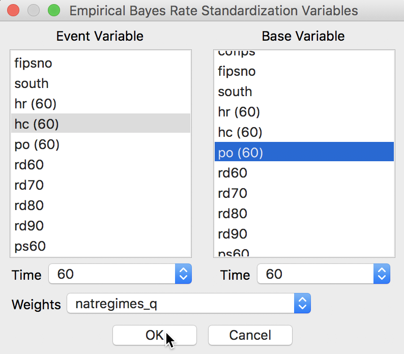
Figure 14: EBI Moran scatter plot variable selection
This yields the Moran scatter plot shown in Figure 15. The axes labels show the numerator and denominator of the rates for which the statistic was computed. In our example, the result is a spatial autocorrelation coefficient of 0.518. Using permutation inference (not shown) with 999 permutations yields a pseudo p-value of 0.001 with an associated z-value of 48.7. All standard options for the Moran scatter plot apply (and will not be reviewed).
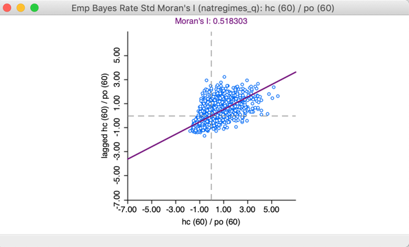
Figure 15: EBI Moran scatter plot
For comparison purposes, we also compute Moran’s I for the crude rate, hr(60) (using the same queen contiguity spatial weights). The result, shown in Figure 16 yields a spatial autocorrelation coefficient of 0.369, quite a bit lower in absolute magnitude. This coefficient remains highly significant at 0.001 with a z-value of 33.7.
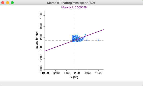
Figure 16: Moran scatter plot for the raw rate
Note that the inference for the raw rate may be somewhat misleading since it ignores the intrinsic variance instability of the rates. In a strict sense, the Moran’s I test for spatial autocorrelation is based on an assumption of a constant mean (obtained by de-meaning the variables) and a constant variance. The latter is violated in the case of rates. The EBI transformation ensures that this does not affect the resulting inference.
Saving the results
A slight difference with the options for the standard Moran scatter plot pertains to the Save Results item. An additional option allows for the transformed rates to be added to the data table. The values are the actual EBI rates, not their standardized form that is used in the computation of Moran’s I. The results are identical to what would be obtained using the Rates option in the Table Calculator. The option is given as EB Rates in Figure 17.
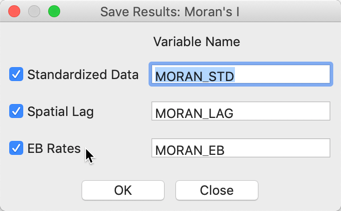
Figure 17: Save EB rates
References
Anselin, Luc, Nancy Lozano-Gracia, and Julia Koschinky. 2006. “Rate Transformations and Smoothing.” Technical Report. Urbana, IL: Spatial Analysis Laboratory, Department of Geography, University of Illinois.
Anselin, Luc, Ibnu Syabri, and Oleg Smirnov. 2002. “Visualizing Multivariate Spatial Correlation with Dynamically Linked Windows.” In New Tools for Spatial Data Analysis: Proceedings of the Specialist Meeting, edited by Luc Anselin and Sergio Rey. University of California, Santa Barbara: Center for Spatially Integrated Social Science (CSISS).
Assunção, Renato, and Edna A. Reis. 1999. “A New Proposal to Adjust Moran’s I for Population Density.” Statistics in Medicine 18: 2147–61.
Lee, Sang-Il. 2001. “Developing a Bivariate Spatial Association Measure: An Integration of Pearson’s r and Moran’s I.” Journal of Geographical Systems 3: 369–85.
Marshall, R. J. 1991. “Mapping Disease and Mortality Rates Using Empirical Bayes Estimators.” Applied Statistics 40: 283–94.
-
University of Chicago, Center for Spatial Data Science – anselin@uchicago.edu↩
-
In the case of the regression of \(x\) on \(Wx\), the explanatory variable \(Wx\) is endogenous, so that the ordinary least squares estimation of the linear fit is biased. However, with \(Wy\) referring to a different variable, the so-called simultaneous equation bias is a non-issue.↩
-
Using the default random seed, this yields a z-value of 41.4.↩
-
The specific steps have been illustrated extensively in previous Chapters.↩
-
In practice, once the data set contains over 1,000 observations, even very small spatial correlation coefficients tend to turn out to be significant. This is a consequence of the variance becoming smaller with larger sample sizes. It is an issue comparable to the situation in a regression with a large number of observations when all coefficients will tend to be significant.↩