Dimension Reduction Methods (2)

Distance Preserving Methods

Introduction

In this chapter, we continue our review of ways to reduce the variable dimension of a problem, but now focus on so-called distance preserving methods, i.e., techniques that attempt to represent, or, more precisely, embed data points from a high-dimensional attribute space in a lower dimensional space (typically 2D or 3D) for easy visualization. This representation is such that the relative distances between the data points are preserved as much as possible. We focus on two methods, the classic multidimensional scaling (MDS) and the more recently developed t-SNE, a variant of a principle referred to as stochastic neighbor embedding. While MDS is a linear technique, t-SNE may be more appropriate in the case when the relationships among the variables may be nonlinear. Also, MDS tends to assure that points that are far apart in high-dimensional space are also far apart in the lower-dimensional space, whereas t-SNE is more attuned at preserving the relative location of close points.

For each method, we first present some basic concepts and the implementation in GeoDa. We then consider more specifically a spatialized approach, where we exploit geovisualization, linking and brushing to explore the connection between neighbors in multi-attribute space and neighbors in geographic space.

To illustrate these techniques, we continue to use the Guerry data set on moral statistics in 1830 France, which comes pre-installed with GeoDa.

Objectives

• Understand the mathematics behind classic metric multidimensional scaling (MDS)

• Understand the principle behind the SMACOF algorithm

• Carry out multidimensional scaling for a set of variables

• Gain insight into the various options used in MDS analysis

• Interpret the results of MDS

• Understand the mathematical principles behind t-SNE

• Carry out t-SNE to visualize multi-attribute data

• Understand the role of the various t-SNE optimization parameters

• Interpret the results of t-SNE

• Compare closeness in attribute space to closeness in geographic space

• Carry out local neighbor match test using MDS neighbors

GeoDa functions covered

• Clusters > MDS
  • select variables
  • MDS methods
  • MDS parameters
  • saving MDS results
  • spatial weights from MDS results
• Clusters > t-SNE
  • select variables
  • t-SNE optimization parameters
  • saving t-SNE results
  • spatial weights from t-SNE results
• Weights Manager
  • weights intersection
• Space > Local Neighbor Match Test

Multidimensional Scaling (MDS)

Principle

Multidimensional Scaling or MDS is a classic multivariate approach designed to portray the embedding of a high-dimensional data cloud in a lower dimension, typically 2D or 3D. The technique goes back to pioneering work on so-called metric scaling by Torgerson (Torgerson 1952, 1958), and its extension to non-metric scaling by Shepard and Kruskal (Shepard 1962a, 1962b; Kruskal 1964). A very nice overview of the principles and historical evolution of MDS as well as a more complete list of the classic references can be found in Mead (1992).

MDS is based on the notion of distance between observation points in multiattribute space. For \(k\) variables, the Euclidean distance between observations \(x_i\) and \(x_j\) in \(k\)-dimensional space is \[d_{ij} = || x_i - x_j|| = [\sum_{h=1}^k (x_{ih} - x_{jh})^2]^{1/2},\] the square root of the sum of the squared differences between two data points over each variable dimension. In this expression, \(x_i\) and \(x_j\) are \(k\)-dimensional column vectors, with one value for each of the \(k\) variables (dimensions). In practice, it turns out that working with the squared distance is mathematically more convenient, and it does not affect the properties of the method. In order to keep the notation straight, we will use \(d_{ij}^2\) for the squared distance.

The squared distance can also be expressed as the inner product of the difference between two vectors: \[d_{ij}^2 = (x_i - x_j)'(x_i - x_j),\]

with \(x_i\) and \(x_j\) represented as \(k \times 1\) column vectors. It is important to keep the dimensions straight, since the data points are typically contained in an \(n \times k\) matrix \(X\), where each observation corresponds to a row of the matrix. However, in order to obtain the sum of squared differences as a inner product, each observation (on the \(k\) variables) must be represented as a column vector.

An alternative to Euclidean distance is a Manhattan (city block) distance, which is less susceptible to outliers, but does not lend itself to being expressed as an inner product of two vectors: \[d_{ij} = \sum_{h=1}^k |x_{ih} - x_{jh}|,\] the sum of the absolute differences in each dimension.

The objective of MDS is to find the coordinates of data points \(z_1, z_2, \dots, z_n\) in 2D or 3D that mimic the distance in multiattribute space as closely as possible. This can be thought of as minimizing a stress function, \(S(z)\): \[S(z) = \sum_i \sum_j (d_{ij} - ||z_i - z_j||)^2.\] In other words, a set of coordinates in a lower dimension (\(z_i\), for \(i = 1, \dots, n\)) are found such that the distances between the resulting pairs of points ( \(||z_i - z_j||\) ) are as close as possible to their pair-wise distances in high-dimensional multi-attribute space ( \(d_{ij}\) ). Note that, due to the use of a squared difference, this objective functions penalizes large differentials more. Hence a tendency of MDS to represent points that are far apart rather well, but maybe with less attention to points that are closer together.

Mathematical details

Classic metric scaling

Classic metric MDS, one of the two methods implemented in GeoDa, approaches the optimization problem indirectly by focusing on the cross product between the actual vectors of observations \(x_i\) and \(x_j\) rather than between their difference, i.e., the cross-product between each pair of rows in the observation matrix \(X\). The values for all these cross-products are contained in the matrix expression \(XX'\). Note that this matrix, often referred to as a Gram matrix, is of dimension \(n \times n\) (and not \(k \times k\) as is the case for the more familiar \(X'X\) used in PCA).

If the actual observation matrix \(X\) is available, then the eigenvalue decomposition of the Gram matrix provides the solution to MDS. In the same notation as used for PCA (but now pertaining to the matrix \(XX'\)): \[XX' = VGV',\] where V is the matrix with eigenvectors (each of dimension \(n \times 1\)) and \(G\) is a \(n \times n\) diagonal matrix that contains the eigenvalues on the diagonal. It turns out that the new coordinates are found as: \[Z = VG^{1/2},\] i.e., each eigenvector (for \(n\) observations) is multiplied by the square root of the matching eigenvalue, with the eigenvalues ordered in decreasing order. Typically, only the first two or three columns of \(VG^{1/2}\) are used. This also implies that only the first few (largest) eigenvalues need to be computed, rather than the full set of \(n\) (see the Appendix for details).

More generally, MDS only requires the specification of a dissimilarity or squared distance matrix \(D^2\), not necessarily the full set of observations \(X\). As it turns out, the Gram matrix can be obtained from \(D^2\) by double centering: \[XX' = - \frac{1}{2} (I - M)D^2(I - M),\] where \(M\) is the \(n \times n\) matrix \((1/n)\iota \iota'\) and \(\iota\) is a \(n \times 1\) vector of ones (so, \(M\) is an \(n \times n\) matrix containing 1/n in every cell). The matrix \((I - M)\) converts values into deviations from the mean. In the literature, the joint pre- and post-multiplication by \((I - M)\) is referred to as double centering.

Given this equivalence, we don’t actually need the matrix \(X\) (in order to construct \(XX'\)) since the eigenvalue decomposition can be applied directly to the double centered squared distance matrix (see the Appendix). A more formal explanation of the mathematical properties can be found in Borg and Groenen (2005), Chapter 7, and Lee and Verleysen (2007), pp. 74-78.

SMACOF

SMACOF stands for “scaling by majorizing a complex function,” and was initially suggested by de Leeuw (1977) as an alternative to the gradient descent method that was typically employed to minimize the MDS stress function. It was motivated in part because the eigenvalue approach outlined above for classic metric MDS does not work unless the distance function is Euclidean. In many early applications of MDS in psychometrics this was not the case.

The idea behind the iterative majorization method is actually fairly straightforward, but its implementation in this particular case is quite complex.² In essence, a majorizing function is found that is much simpler than the original function, and, for a minimization problem, is always above the actual function. With a function \(f(x)\), a majorizing function \(g(x,z)\) is such that for a fixed point \(z\) the two functions are equal, such that \(f(z) = g(z,z)\) (\(z\) is called the supporting point). The auxiliary function should be easy to minimize (easier than \(f(x)\)) and always dominate the original function, such that \(f(x) \leq g(x,z)\). This leads to the so-called sandwich inequality (coined as such by de Leeuw): \[f(x^*) \leq g(x^*,z) \leq g(z,z) = f(z),\] where \(x^*\) is the value that minimizes the function \(g\).

The iterative part stands for the way in which one proceeds. One starts with a value \(x_0\), such that \(g (x,x_0) = f(x_0)\). For example, consider a parabola that sits above a complex nonlinear function and touches it at \(x_0\), as shown in Figure 1. We can then easily find the minimum for the parabola, say at \(x_1\). Next, we move a new parabola so that it touches our function at \(x_1\), with again \(g(x,x_1) = f(x_1)\). In the following step, we find the minimum for the new parabola at \(x_2\) and keep proceeding in this iterative fashion until the difference between \(x_k\) and \(x_{k-1}\) for two consecutive steps is less than a critical value (the convergence criterion). At that point we consider the minimum of our parabola to be the same as the minimum for the function \(f(x)\), or, close enough, given our convergence criterion.

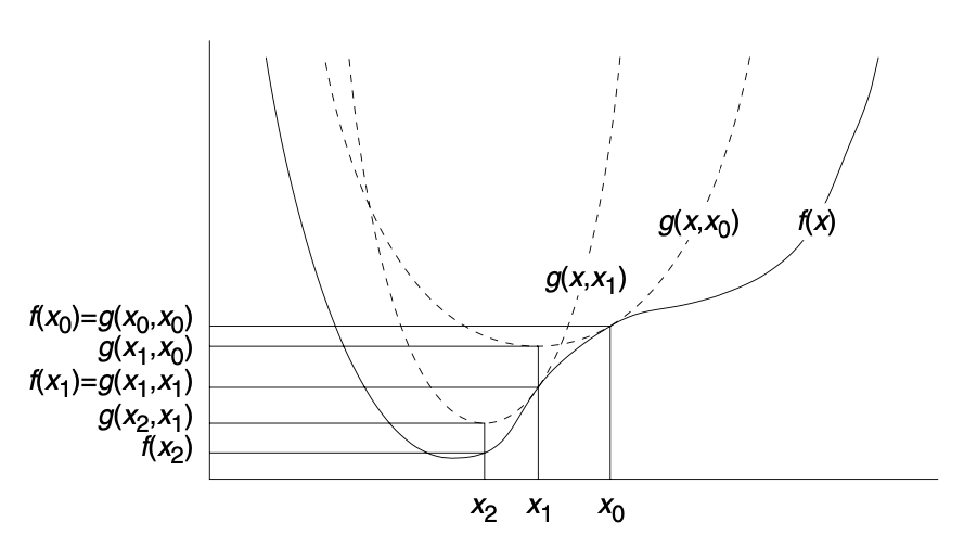
Figure 1: Iterative majorization (source: Borg and Groenen, 2005, p. 180)

In general, the stress function for a solution \(Z\) to the MDS problem can be written as: \[S(Z) = \sum_{i < j} (\delta_{ij} - d_{ij}(Z))^2 = \sum_{i<j} \delta_{ij}^2 + \sum_{i<j} d_{ij}^2(Z) - 2 \sum_{i<j} \delta_{ij}d_{ij}(Z),\] where \(\delta_{ij}\) is the distance between \(i\) and \(j\) for the original configuration, and \(d_{ij}(Z)\) is the corresponding distance for a proposed solution \(Z\). Note that \(\delta_{ij}\) can be based on any distance metric or dissimilarity measure, but \(d_{ij}(Z)\) is a Euclidean distance. In the stress function, the first term is a constant, since it does not change with the values for the coordinates in \(Z\). The second term is a sum of squared distances between pairs of points in \(Z\), and the third term is a weighted sum of the pairwise distances (each weighted by the initial distances).³ We need to find a set of coordinates \(Z\) that minimizes \(S(Z)\).

The upshot of the iterative majorization is the so-called Guttman transform, which expresses an updated solution \(Z\) as a function of a tentative solution to the majorizing condition, \(Y\), through the following equality: \[Z = (1/n)B(Y)Y,\] where the \(n \times n\) matrix \(B(Y)\) has off-diagonal elements \(B_{ij} = - \delta_{ij} / d_{ij}(Y)\), and diagonal elements \(B_{ii} = - \sum_{j, j\neq i} B_{ij}\). Note that this negative of a sum of negatives turns out to be positive. Basically, the diagonal elements equal the sum of the absolute values of all the column/row elements, so that rows and columns sum to zero, i.e., the matrix \(B\) is double centered (details are given in the section on Iterative majorization of the stress function in the Appendix).

In practice, this means that the majorization algorithm proceeds through a number of simple steps:

• start by picking a set of (random) starting values for \(Z\) and set \(Y\) to these values

• compute the stress function for the current value of \(Z\)

• find a new value for \(Z\) by means of the Guttman transform, using the computed distances included in \(B(Y)\), based on the current value of \(Y\)

• update the stress function and check its change; stop when the change is smaller than a pre-set difference

• if no convergence yet, set \(Y\) to the new value of \(Z\) and proceed with the update, etc.

Implementation

Default settings

The MDS functionality in GeoDa is invoked from the Clusters toolbar icon, or from the main menu, as Clusters > MDS. It is the second item in the dimension reduction submenu, as shown in Figure 2.

Figure 2: MDS menu option

This brings up the MDS Settings panel through which the variables are selected and various computational parameters are set. We continue with the same six variables as used previously in the PCA example, i.e., Crm_prs, Crm_prp, Litercy, Donatns, Infants, and Suicids. For now, we leave all options to their default settings, shown in Figure 3. The default method is classic metric with the variables standardized. Since this method only works for Euclidean distances, the Distance Function option is not available. Importantly, the default number of dimensions is set to 2 (see below for 3D MDS).

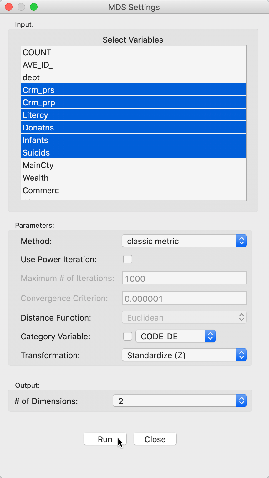
Figure 3: MDS input variable selection

Saving the MDS coordinates

After clicking the Run button, a small dialog is brought up to select the variable names for the new MDS coordinates, in Figure 4.

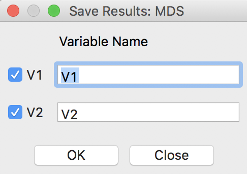
Figure 4: MDS result variable selection

As mentioned, GeoDa offers both the standard 2D MDS as well as a 3D MDS. The default used here is 2D, with the new variables V1 and V2 checked (the coordinates in the new space). In a typical application, the default variable names of V1 and V2 should be changed to a more appropriate choice.

The coordinates are added to the data table, as illustrated for the first five observations in Figure 5.

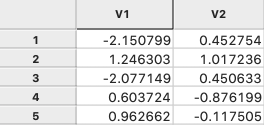
Figure 5: MDS coordinates in data table

With some additional computations, we can verify how these results are obtained. First, we need to create the matrix \(XX'\) from the standardized values for the six variables. Next, we compute the eigenvalues and eigenvectors for this \(85 \times 85\) matrix.⁴ The results are summarized in Figure 6.

The top row shows the first two eigenvalues, with their square roots listed immediately below. The eigenvector elements are also given for the first five observations (out of 85). The columns V1 and V2 give the corresponding MDS coordinates, calculated by multiplying the square root of the eigenvalue with the matching elements of the eigenvector (see the mathematical derivation in Classic metric scaling). The results are the same as those reported in Figure 5.

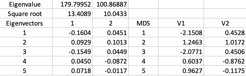
Figure 6: MDS coordinate calculations

MDS scatter plot

After the variable selection, OK generates a two-dimensional scatter plot with the observations, illustrated in Figure 7. In this scatter plot, points that are close together in two dimensions should also be close together in the six-dimensional attribute space. In addition, two new variables with the coordinate values will be added to the data table (as usual, to make this addition permanent, we need to save the table). Below the scatter plot are two lines with statistics. They can be removed by turning the option View > Statistics off (the default is on).

The statistics list the variables included in the analysis and two rough measures of fit. One is the value of the stress function for the solution, in our example, this is 0.343 (a lower value indicates a better fit). The other is the rank correlation between the distances in multi-attribute space and the distances in the lower-dimensional space, here 0.825 (a higher value suggests a stronger correlation between the relative ranks of the distances). The method used (classic metric) is included in the window top banner.

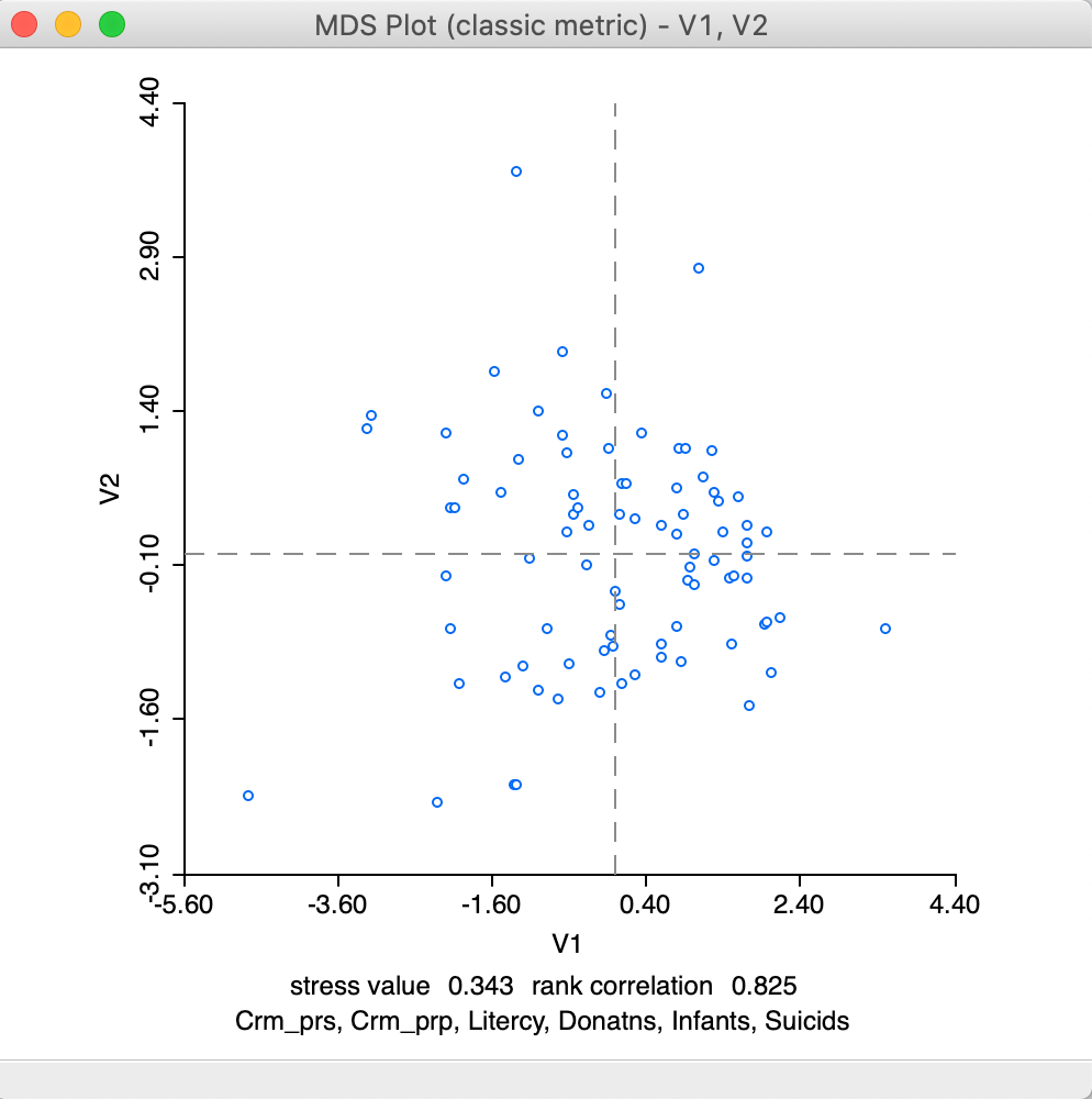
Figure 7: MDS plot

To illustrate the mathematical similarity between PCA and classic metric MDS, consider the scatter plot of the first two principal components (using the same six variables) next to the MDS plot (here shown without the statistics), as in Figure 8. Both plots have the same shape, except for being flipped around the x-axis.

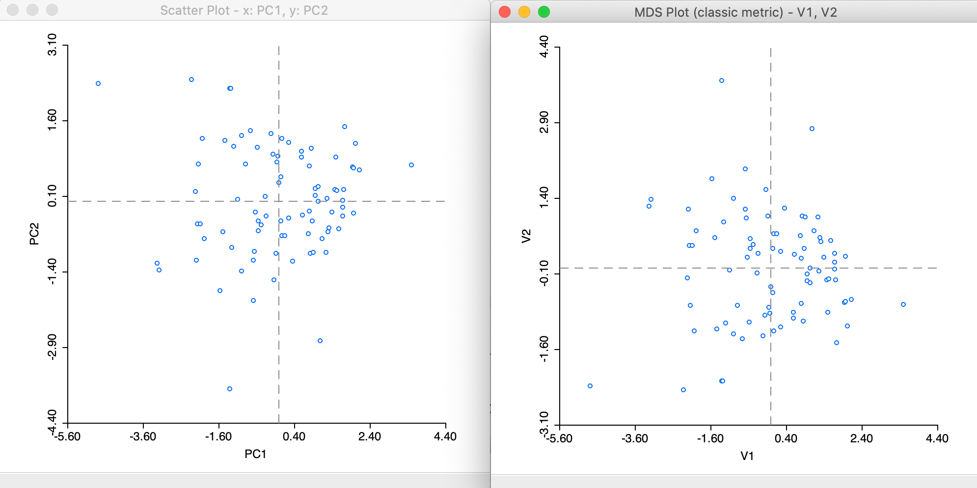
Figure 8: PCA and MDS scatter plots

This is further highlighted by selecting the upper-left quadrant in the PCA plot. The matching points in the MDS plot are in the lower-left quadrant in Figure 9.

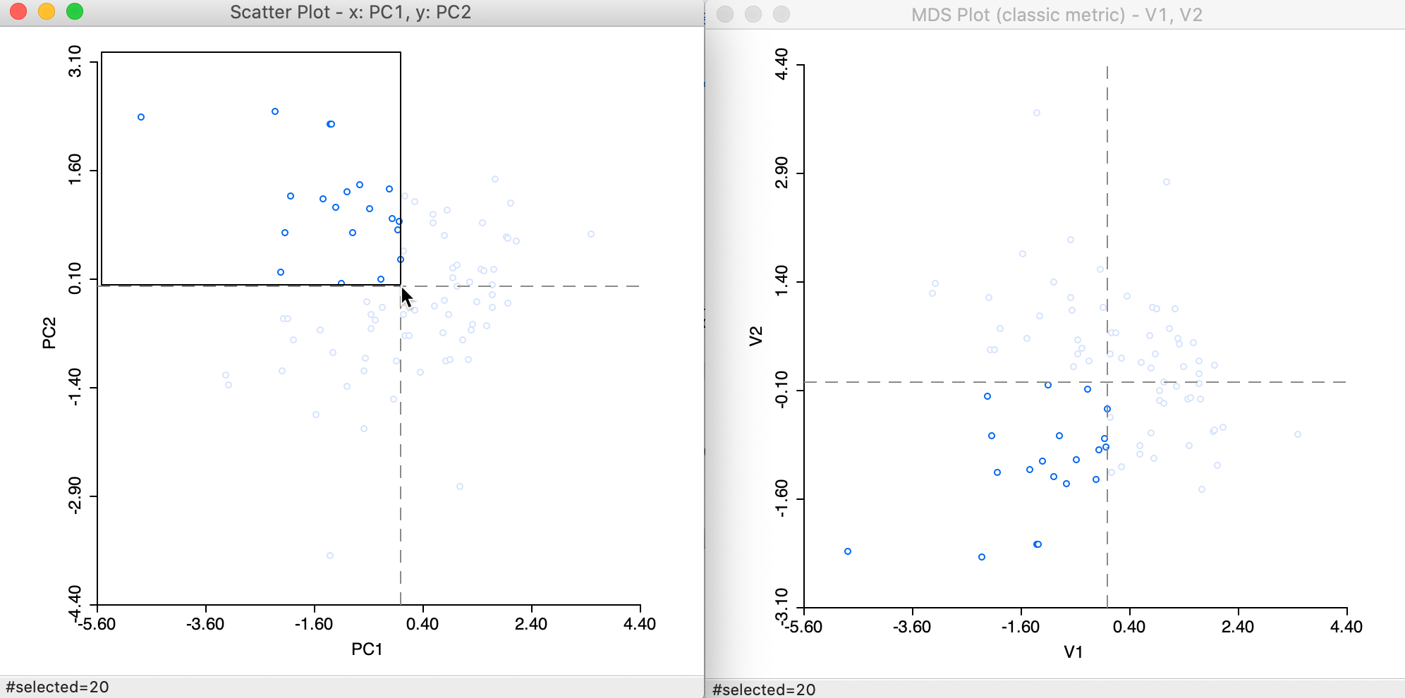
Figure 9: Selected points in PCA and MDS scatter plots

Recall that the signs of the elements of the eigenvectors depend on the computational approach, so that the relative positioning is really what counts. Consequently, points (observations) that are close in MDS space, will also be close in PCA space, and vice versa.

3D MDS

When the # of Dimensions option is set to 3, the results of MDS are visualized in a 3-dimensional scatterplot cube, as in Figure 10. Both the stress value (0.196) as well as the rank correlation (0.931) are superior to the two-dimensional solution. This is to be expected, since less dimension reduction is involved.⁵

Points that are close in the 2D MDS scatter plot are not necessarily close in 3D. In Figure 10, this seems to be the case, since the three close points selected in the 2D graph on the right also look close in 3D (the points highlighted in yellow).

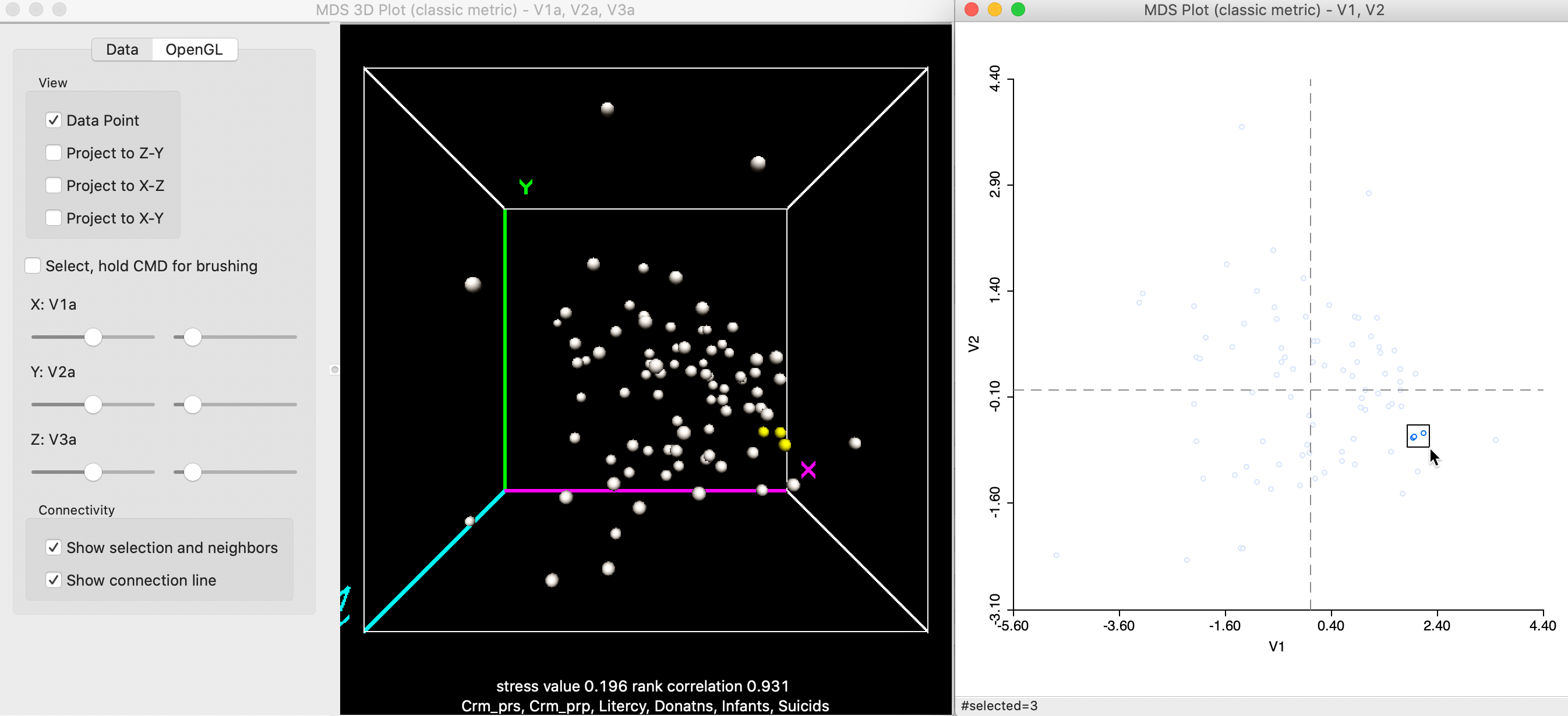
Figure 10: Selected points in 3D and 2D MDS scatter plots (a)

However, this is not necessarily the case, and it is important to take advantage of the rotation of the 3D scatterplot cube to get a better sense of the location of the points in three dimensions. For example, the two points selected in the 2D plot in Figure 11 turn out not to be that close in 3D, after some rotation of the cube.

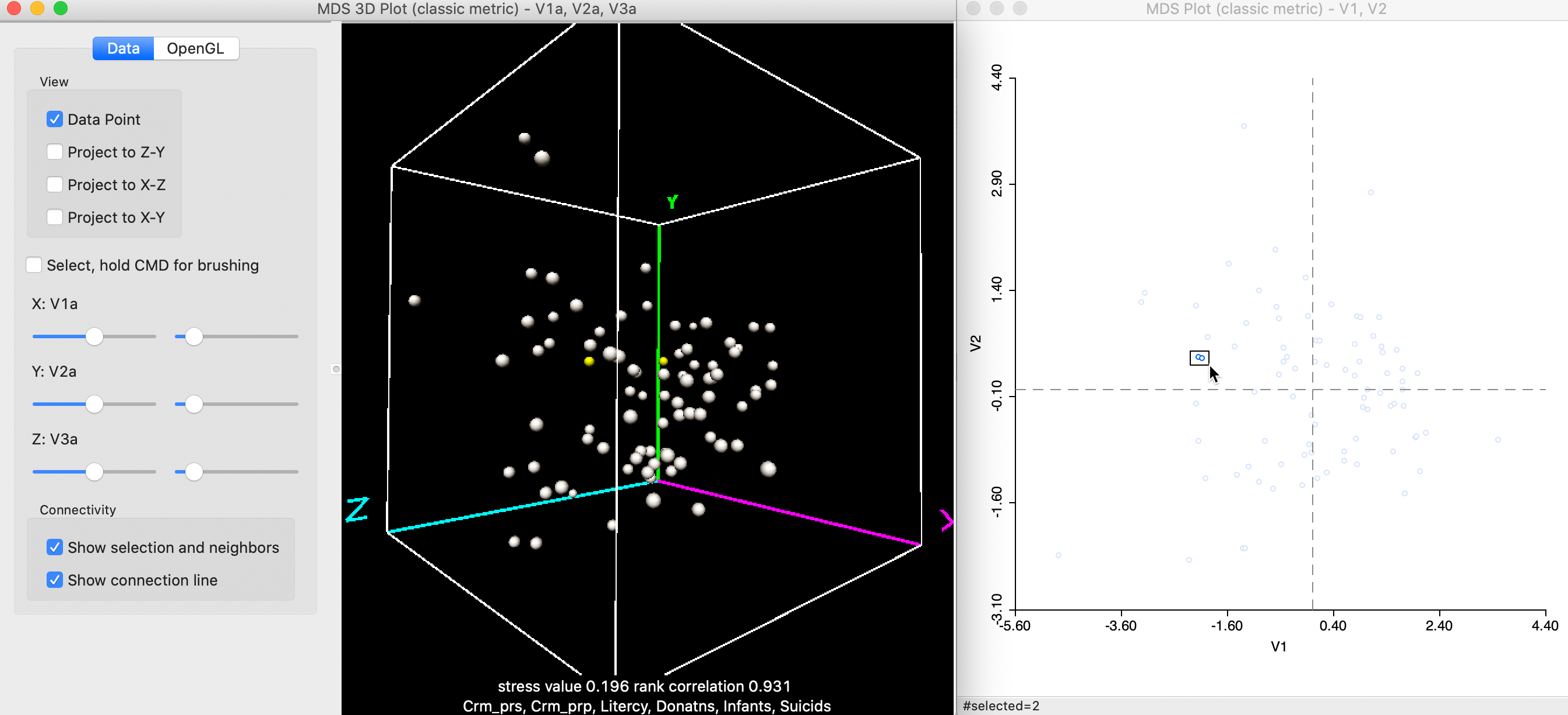
Figure 11: Selected points in 3D and 2D MDS scatter plots (b)

In our typical applications, we will focus on the 2D visualization.

Power approximation

The Parameters panel in the MDS Settings dialog allows for a number of options to be set. The Transformation options are the same as for PCA, with the default set to Standardize (Z), but Standardize (MAD), Raw, Demean, Range Adjust and Range Standardize are available as well. Best practice is to use the variables in standardized form, either the traditional z-transformation, or a more robust alternative (MAD or range standardize).

An option that is particularly useful in larger data sets is to use a Power Iteration to approximate the first few largest eigenvalues needed for the MDS algorithm. Since the first two or three eigenvalue/eigenvector pairs are all that is needed for the classic metric implementation, this provides considerable computational advantages in large data sets. Recall that the matrix for which the eigenvalues/eigenvectors need to be obtained is of dimension \(n \times n\). For large \(n\), the standard eigenvalue calculation will tend to break down.

The Power Iteration option is selected by checking the box in the Parameters panel, as in Figure 12. This also activates the Maximum # of Iterations option. The default is set to 1000, which should be fine in most situations. However, if needed, it can be adjusted by entering a different value in the corresponding box.

Figure 12: MDS power iteration option

At first sight, the result in Figure 13 may seem different from the standard output in Figure 7, but this is due to the indeterminacy of the signs of the eigenvectors. The stress value and rank correlation statistics are identical to the default solution. This is not unexpected, since \(n = 85\) in our example, so that the power approximation is actually not needed.

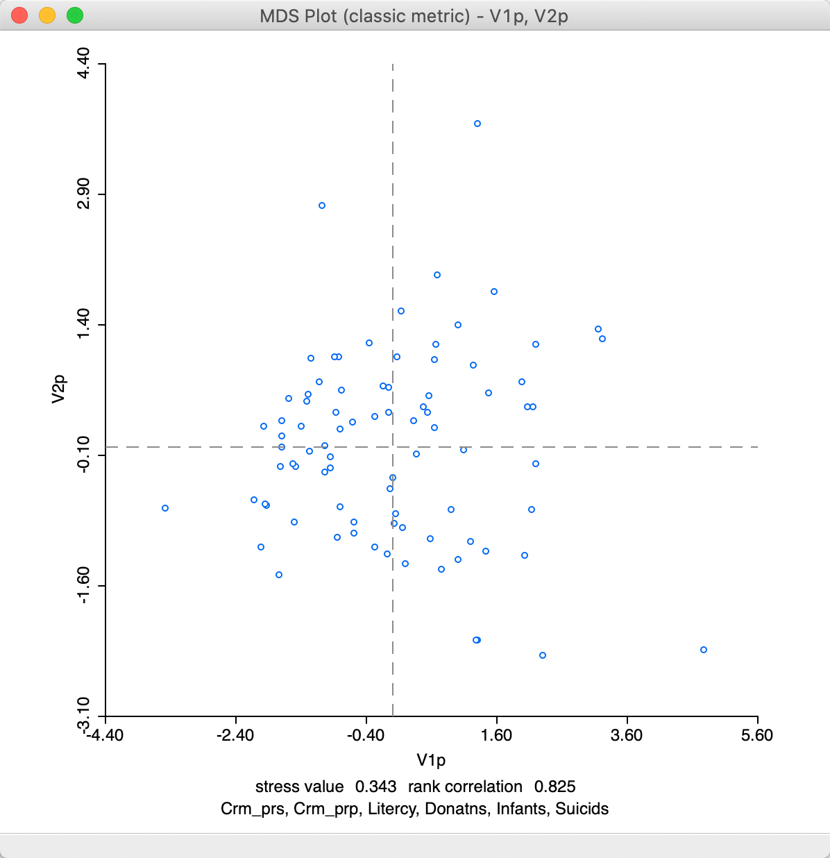
Figure 13: MDS plot (power approximation)

Closer inspection of the two graphs suggests that the axes are flipped. We can clearly see this by selecting the points in the upper right quadrant in the power graph and locating them in the other, as in Figure 14. The relative position of the points is the same in the two graphs, but they are on opposite sides of the y-axis.

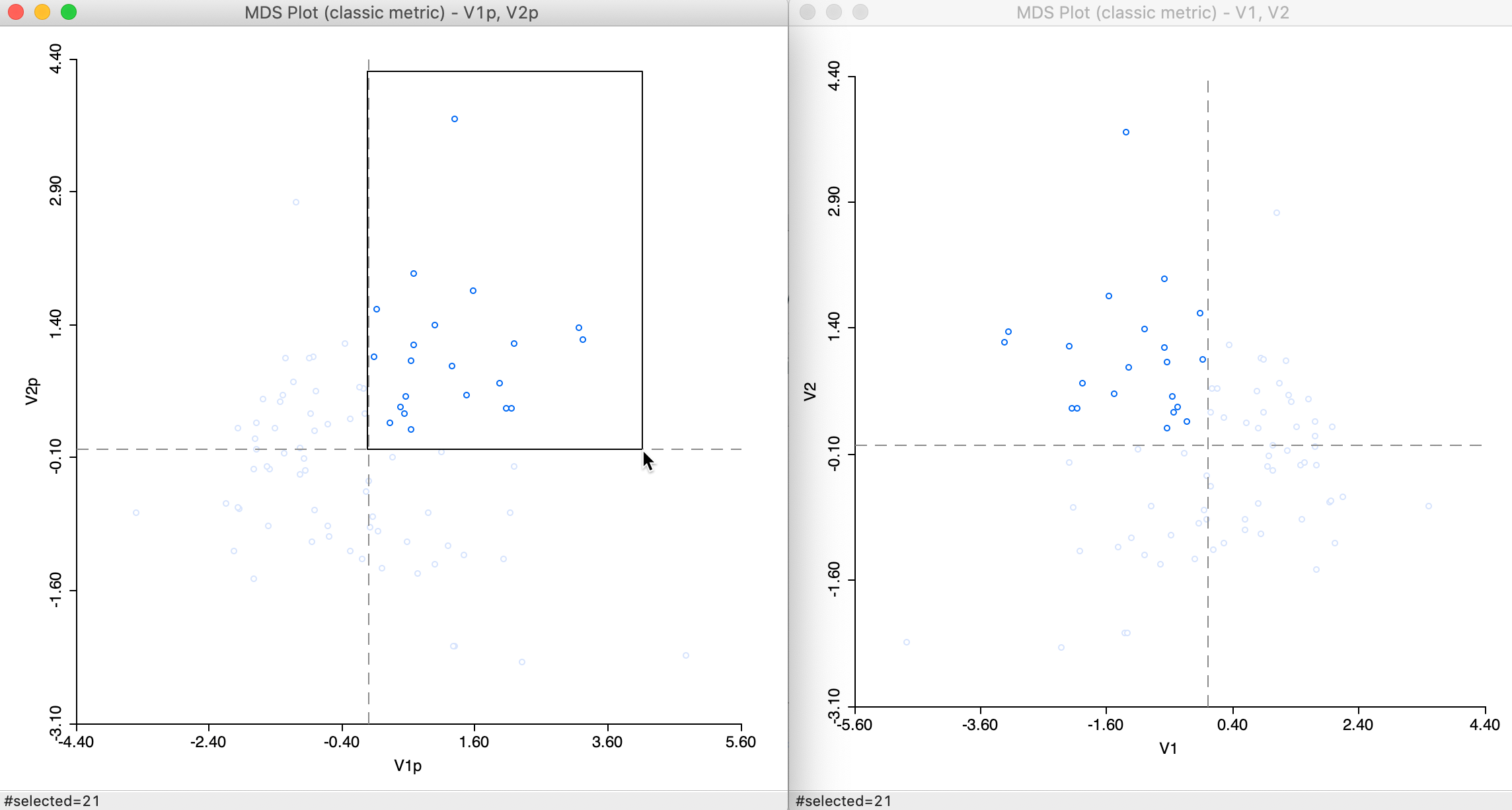
Figure 14: Computation algorithm comparison

SMACOF

The Method option provides two approaches to minimize the stress function. The default is classic metric, but the smacof method is provided as an alternative. When the latter is selected, as in Figure 15, the Maximum # of iterations and the Convergence Criterion can be changed as well (those options are not available to the default classic metric method). The default setting is for 1000 iterations and a convergence criterion of 0.000001. These should be fine for most applications, but they may need to be adjusted if the minimization is not accomplished by the maximum number of iterations.

Figure 15: SMACOF method

As before, after selecting variable names for the two dimensions, a scatter plot is provided (it lists the method in the banner). For our example, the results are as in Figure 16, with the statistics listed at the bottom.

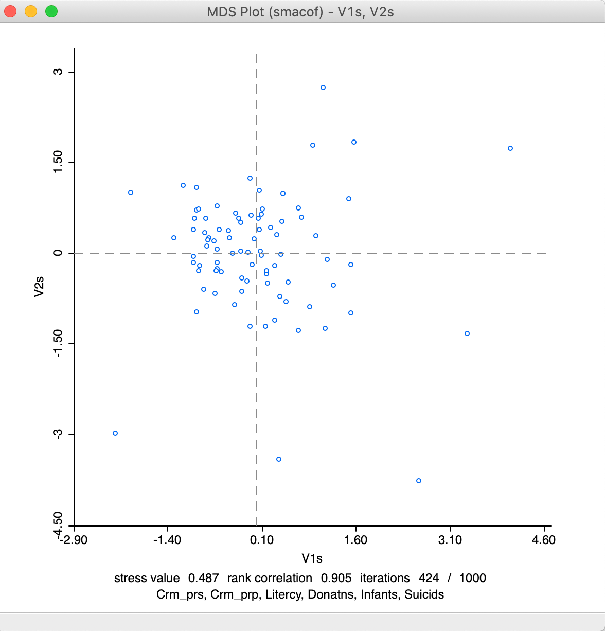
Figure 16: MDS plot using smacof method

Relative to the results for the classic metric method, the stress value is poorer, at 0.487, but the rank correlation is better, at 0.905. It is also shown that convergence (for the default criterion) is reached after 424 iterations. If the result would show 1000/1000 iterations, that would indicate that convergence has not been reached. This means that the default number of iterations would need to be increased. Alternatively, the convergence criterion could be relaxed, but that is not recommended.

We can compare the relative position of the points obtained by means of each method through linking and brushing, in the usual way. For example, in Figure 17 some close points in the SMACOF solution are shown to be somewhat farther apart in the classic metric solution.

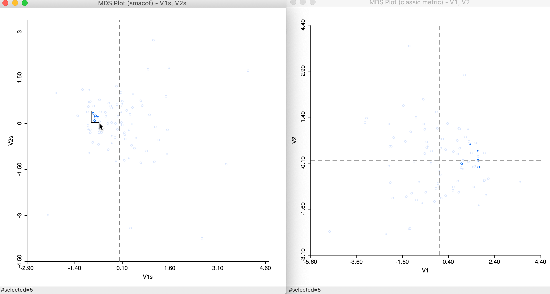
Figure 17: Selected points in SMACOF and classic metric scatter plots

With the smacof method selected, it is now possible to choose an alternative distance metric for the original points, such as the Manhattan block distance. This computes absolute differences instead of squared differences. The option is shown in Figure 18. The effect is to lessen the impact of outliers, or large distances in the original high dimensional space.

Figure 18: SMACOF Manhattan distance function

The result that follows from a Manhattan distance metric is quite different from the default Euclidean SMACOF plot. As seen in Figure 19, the scale of the coordinates is different. Note that the range of values for V1sm and V2sm is much smaller than for the metric plot, so even if the points look farther apart, they are actually quite close on the scale of Figure 16. However, the identification of close observations can also differ quite a bit between the two plots. This can be further explored using linking and brushing (not shown).

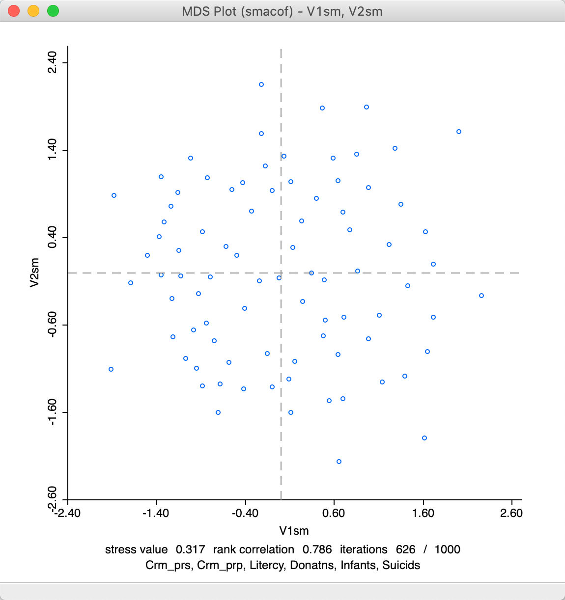
Figure 19: SMACOF plot for Manhattan distance

Note that in terms of fit, the stress value of 0.317 is better than for SMACOF with Euclidean distance, but the rank correlation of 0.786 is worse. Convergence is obtained after 626 iterations, slightly more than for the Euclidean distance option.

The moral of the story is that the MDS scatter plots should not be interpreted in a mechanical way, but careful linking and brushing should explore the trade-offs between the different options.

Categorical variable

The MDS interface includes an option to visualize the position of data points that correspond to a particular category. One of the main uses of embedding methods is to discover hidden structure in high-dimensional data, such as particular groupings. The Category Variable option provides a way to visualize how the points that correspond to pre-defined groups in the data position themselves in the lower dimensional embedding. For example, in Figure 20, the Category Variable was set to Region, five broad regions of France, as defined in the Guerry data set (see also the left-hand panel of Figure 36).

Figure 20: MDS categorical variable selection

As a result, after the variable names are entered, the resulting MDS scatter plot designates each point with a color corresponding to its category, as in Figure 21. This primarily for visualization during the exploratory process. An alternative way to assess the way the point locations might correspond to different groups is given in the section on Visualizing a categorical variable, discussed in the context of t-SNE, but equally applicable to MDS scatter plots.

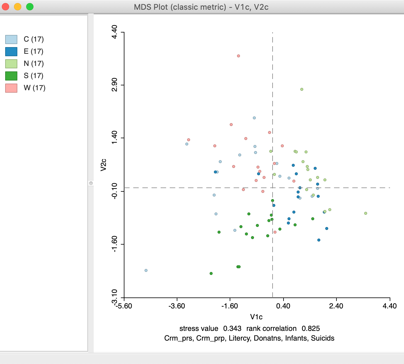
Figure 21: MDS scatter plot with categorical variables

Interpretation

In a general sense, the multidimensional scaling method essentially projects points from a high-dimensional multivariate attribute space onto a two or three-dimensional space. To get a more precise idea of how this process operates, we can link points that are close in the MDS scatter plot to the matching lines in a parallel coordinate plot. Data points that are close in multidimensional variable space should be represented by lines that are close in the PCP.

In Figure 22, we selected two points that are close in the MDS scatter plot and assess the matching lines in the six-variable PCP. Since the MDS works on standardized variables, we have expressed the PCP in those dimensions as well by means of the Data > View Standardized Data option. While the lines track each other closely, the match is not perfect, and is better on some dimensions than on others. For example, for Crm_prp and Suicids, the values are near identical, whereas for Infants the gap between the two values is quite large.

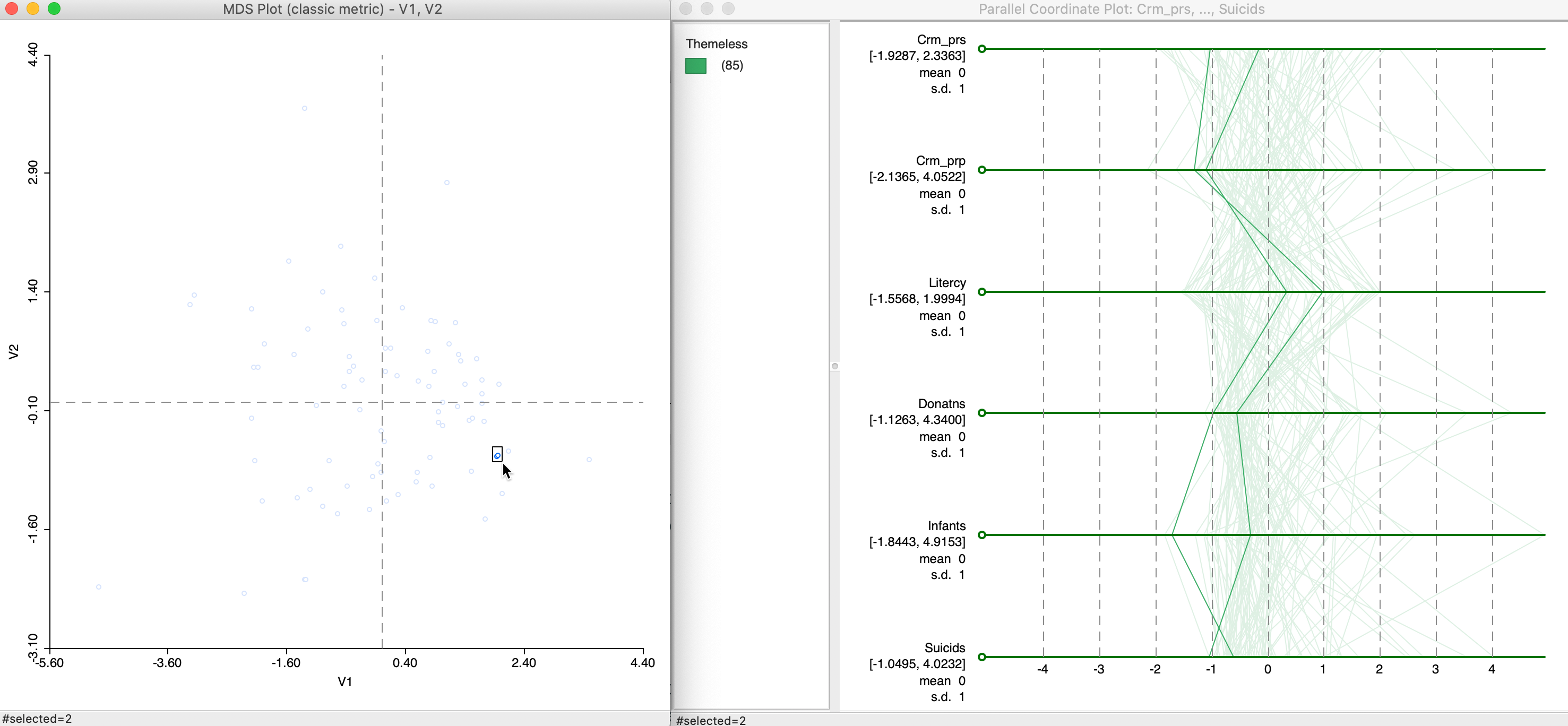
Figure 22: MDS and PCP, close points

To provide some context, Figure 23 provides an example of two points that are far from each other in the MDS plot (in the top and bottom of the left hand panel). The gaps between the PCP lines are generally much farther from each other, although for Litercy and Infants, they are quite close.

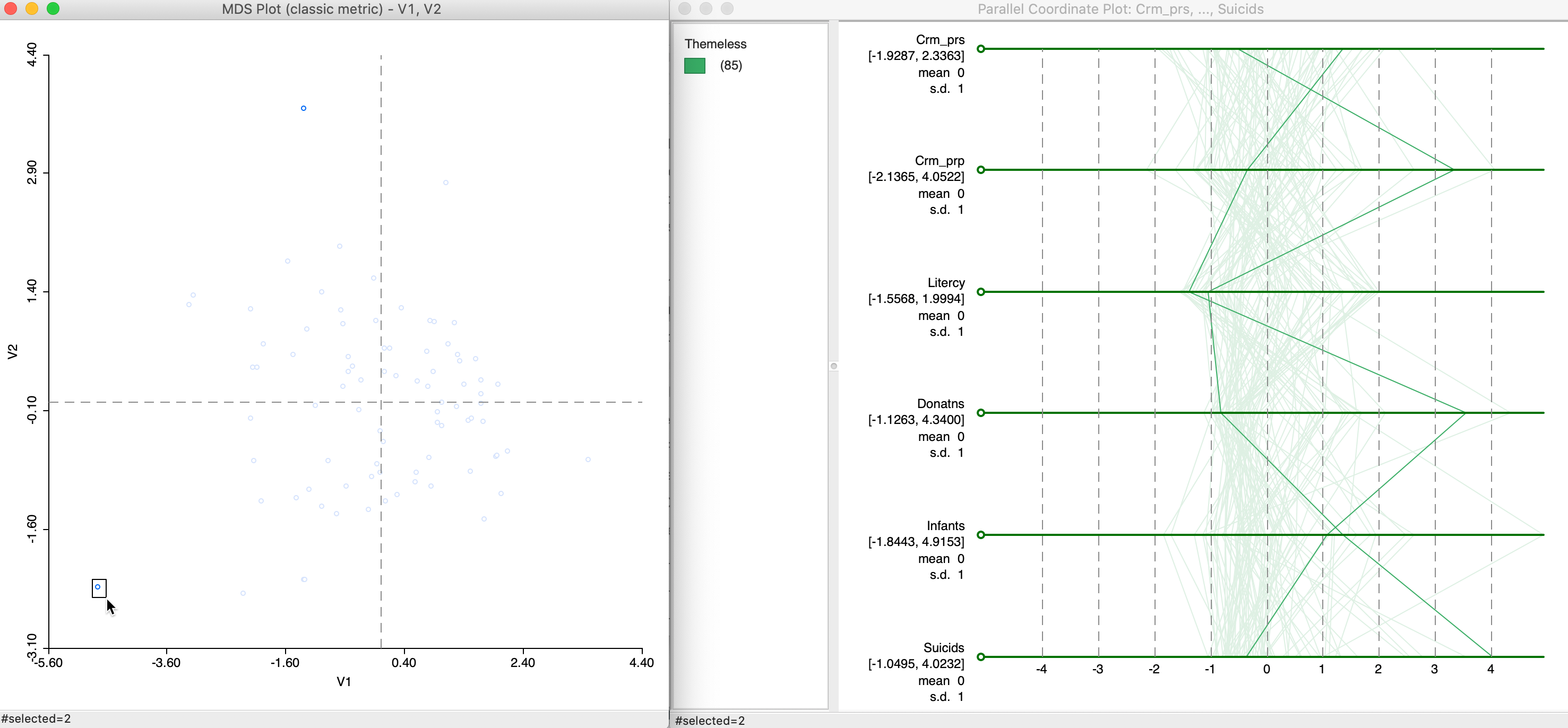
Figure 23: MDS and PCP, remote points

For a proper interpretation, this needs to be examined more carefully, for example, by brushing the MDS scatter plot, or, alternatively, by brushing the PCP and examining the relative locations of the matching points in the MDS scatter plot.

t-SNE

Principle

A drawback of a linear dimension reduction technique like MDS is that it tends to do less well to keep the low-dimensional representation of similar data points close together. t-SNE is an alternative technique that addresses this aspect. It was originally outlined in van der Maaten and Hinton (2008) as a refinement of the stochastic neighbor embedding (SNE) idea formulated by Hinton and Roweis (2003).

Instead of basing the alignment between high and low-dimensional representations on a stress function that includes the actual distances, the problem is reformulated as one of matching two different probability distributions. These distributions are conditional probabilities that represent similarities between data points. More precisely, a conditional probability for the original high-dimensional data of \(p (j | i)\) expresses the probability that \(j\) is picked as a neighbor of \(i\). In other words, the distance between \(i\) and \(j\) is converted into a probability measure using a kernel centered on \(i\). The kernel is a symmetric distribution such that the probability decreases with distance. For example, using a normal (Gaussian) distribution centered at \(i\) with a variance of \(\sigma_i^2\) would yield the conditional distribution as: \[ p_{j|i} = \frac{exp(-d(x_i,x_j)^2/\sigma_i^2)}{\sum_{h \neq i} exp(-d(x_i,x_h)^2/\sigma_i^2) },\] with \(d(x_i, x_j) = ||x_i - x_j||\), i.e., the Euclidean distance between \(i\) and \(j\) in high-dimensional space, and, by convention, \(p_{i|i} = 0\). The variance \(\sigma_i^2\) determines the bandwidth of the kernel and is chosen optimally for each point, such that a target perplexity is reached.

Perplexity is a concept that originates in information theory. It is related to the Shannon entropy of a distribution, \(H = - \sum p_i ln(p_i)\), such that perplexity \(= 2^{H}\). While a complex concept, the perplexity intuitively relates to a smooth measure of the effective number of neighbors (fewer neighbors relates to a smaller perplexity). In regions with dense points, the variance \(\sigma_i^2\) should be smaller, whereas in areas with sparse points, it should be larger to reach the same number of neighbors (something similar in spirit to the adaptive bandwidth to select the \(k\) nearest neighbors).

In t-SNE (as opposed to the original SNE), the conditional probabilities are turned into a joint probability \(P\) as: \[p_{ij} = \frac{p(j|i) + p(i | j)}{2n},\] where \(n\) is the number of observations.

The counterpart of the distribution \(P\) for the high-dimensional points is a distribution \(Q\) for the points in a lower dimension. The innovation behind the t-SNE is that it uses a thick tailed normalized Student-t kernel with a single degree of freedom to avoid some issues associated with the original SNE implementation.⁶ The associated distribution for points \(z_i\) in the low-dimensional space is: \[q_{ij} = \frac{(1 + ||z_i - z_j||^2)^{-1}}{\sum_{h \neq l} (1 + ||z_h - z_l||^2)^{-1}}.\] The measure of fit between the original and embedded distribution is based on information-theoretic concepts, i.e., the Kullback-Leibler divergence between the two distributions (smaller is a better fit): \[C = KLIC(P || Q) = \sum_{i \neq j} p_{ij} \log \frac{p_{ij}}{q_{ij}} = \sum_{i \neq j} [ p_{ij} \log p_{ij} - p_{ij} \log q_{ij} ] .\] In essence, this boils down to trying to match pairs with a high \(p_{ij}\) (nearby points in high dimension) to pairs with a high \(q_{ij}\) (nearby points in the embedded space).

In order to minimize the cost function, we need its gradient. This is the first partial derivative of the function \(C\) with respect to the coordinates \(z_i\). It has the (complex) form: \[\frac{\partial C}{\partial z_i} = 4 \sum_{j \neq i}(p_{ij} - q_{ij})(1 + ||z_i - z_j ||^2)^{-1} (z_i - z_j).\] This simplifies a bit, if we set \(U = \sum_{h \neq l} (1 + ||z_h - z_l||^2)^{-1}\). Therefore, since \(q_{ij} = (1 + ||z_i - z_j ||^2)^{-1} / U\), the term \((1 + ||z_i - z_j ||^2)^{-1}\) can be replaced by \(q_{ij}U\), so that the gradient becomes: \[\frac{\partial C}{\partial z_i} = 4 \sum_{j \neq i}(p_{ij} - q_{ij})q_{ij}U (z_i - z_j).\] The optimization involves a complex gradient search that is adjusted with a learning rate and a momentum term to speed up the process. At each iteration \(t\) the value of \(z_i^t\) is updated as a function of its value at the previous iteration, \(z_i^{t-1}\), a multiplier of the gradient (\(\partial C / \partial z_i\)) represented by the learning rate \(\eta\), and a term that takes into account the change at the previous iteration step, the so-called momentum \(\alpha(t)\) (indexed by \(t\) since it is typically adjusted during the optimization process): \[z_i^t = z_i^{t-1} + \eta \frac{\partial C}{\partial z_i} + \alpha(t)(z_i^{t-1} - z_i^{t-2}).\] The learning rate and momentum are parameters to be specified. In addition, the momentum is typically changed after a number of iterations, which is another parameter that should be set (see Implementation).

The most recent implementation of this optimization process uses advanced algorithms that speed up the process and allow t-SNE to scale to very large data sets, as outlined in van der Maaten (2014) (some details are provided in the Appendix section on Barnes-Hut optimization of t-SNE). The algorithm is rather finicky and may require some trial and error to find a stable solution. An excellent illustration of the sensitivity of the algorithm to various tuning parameters can be found in Wattenberg, Viégas, and Johnson (2016) (https://distill.pub/2016/misread-tsne/).

Implementation

Default settings

The t-SNE functionality is the third option in the dimension reduction section of the cluster toolbar, shown in Figure 24. Alternatively, it can be invoked as Clusters > t-SNE from the menu.

Figure 24: t-SNE menu option

This brings up the main t-SNE interface, in Figure 25. In the left-hand panel is the list of available variables as well as several parameters to fine tune the algorithm. We continue with the same six variables as in the previous examples.

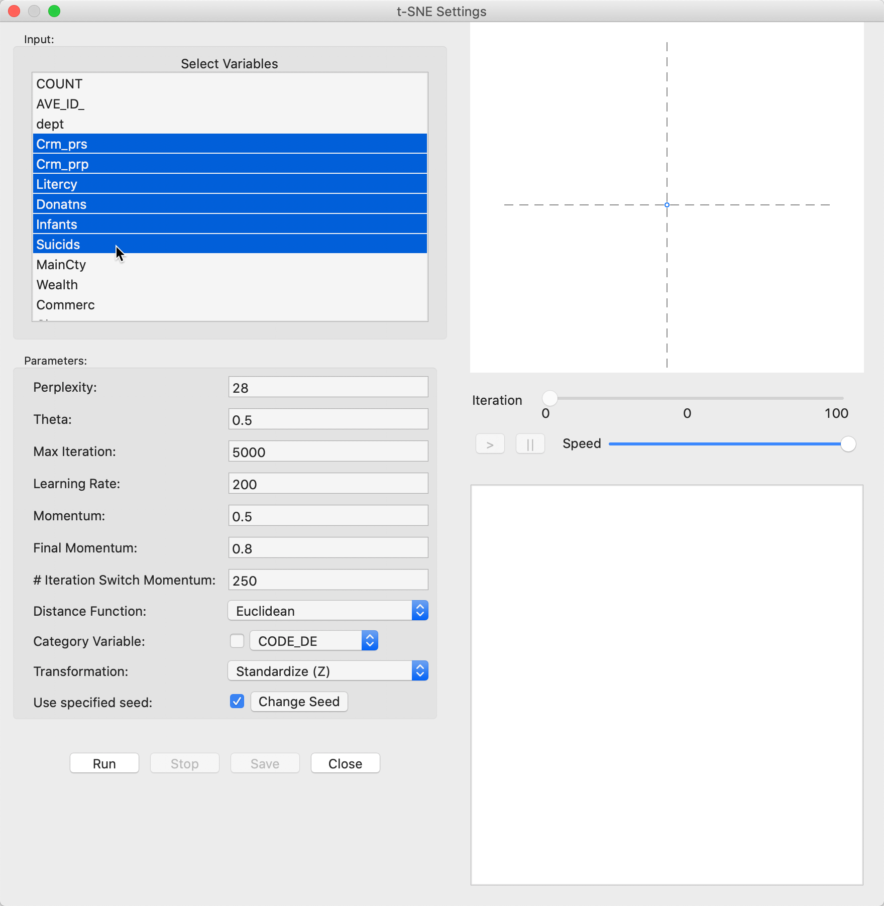
Figure 25: t-SNE variable selection

The right-hand panel consists of a space at the top for the two-dimensional scatterplot with the results shown as the iterations proceed. The bottom panel gives further quantitative information on the quality of every 50 iterations, with a value for the error (i.e., the gradient function), which gives an indication of how the process is converging to a stable state.

In-between the two result panes is a small control panel to adjust the speed of the animation, as well as allowing to pause and resume as the iterations proceed.

With all options left at their default values, pressing Run yields the full set of 5000 iterations, resulting in the scatter plot in Figure 26. The bottom pane indicates a final cost value of 0.241751 and shows that its value has been hovering around 0.241 for the last 100 iterations.⁷

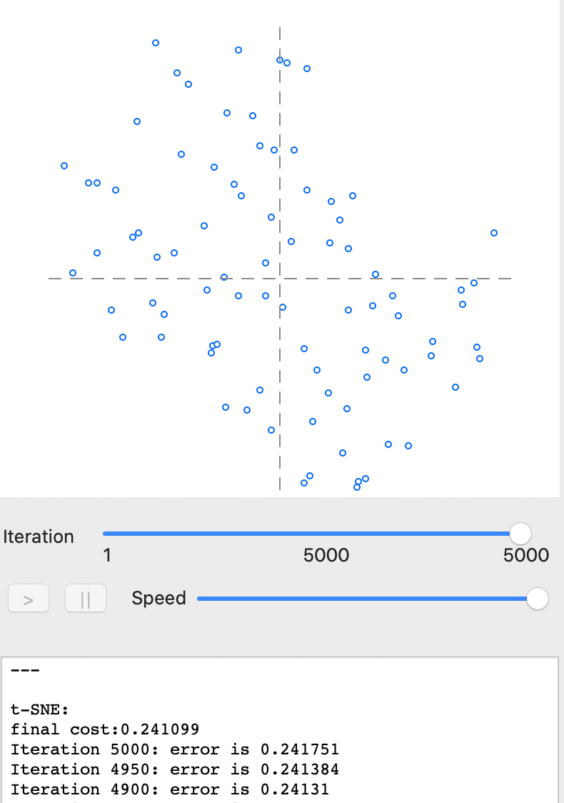
Figure 26: t-SNE results - full iteration

At this point, selecting Save will bring up the customary interface to select variable names for the two dimensions (as in Figure 4). With these specified, the scatter plot is drawn, as in Figure 27. As before, this lists the method in the banner, and contains some summary statistics at the bottom of the graph. These consist of the final cost, the corresponding rank correlation and the number of iterations. Since the t-SNE optimization algorithm is not based on a specific stopping criterion, unless the process is somehow paused (see Animation), the number of iterations will always correspond to what is specified in the options panel. However, this does not mean that it necessarily has resulted in a stable optimum. In practice, one therefore needs to pay close attention to the point pattern of the iterations as they proceed.

The final cost is not comparable to the objective function for MDS, since it is not based on a stress function. On the other hand, the rank correlation is a rough global measure of the correspondence between the relative distances and remains a valid measure. The result of 0.726 is lower than for MDS, but in the same general ball-park as SMACOF with Manhattan distance (see Figure 19). However, it should be kept in mind that t-SNE is geared to optimize local distances, so a global performance measure is not fully appropriate.

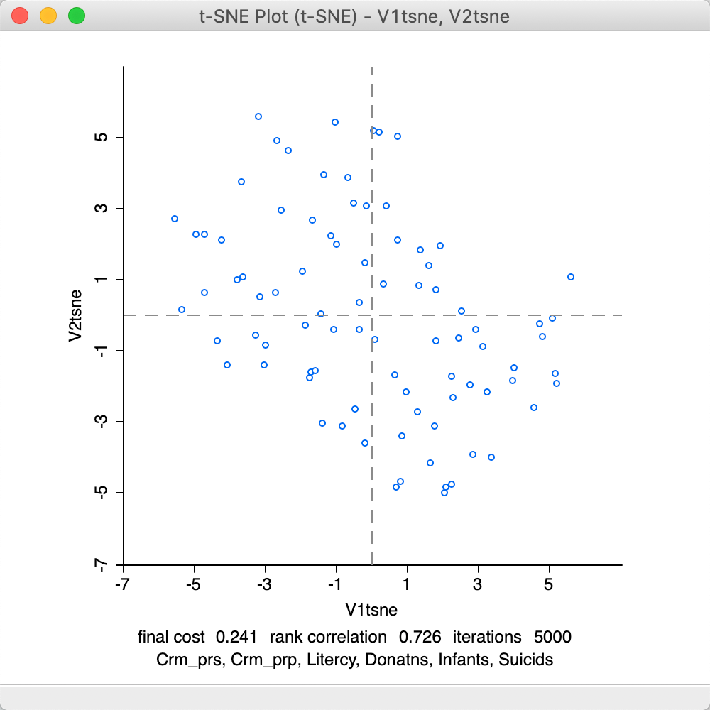
Figure 27: t-SNE default result plot

Animation

As mentioned, with the default settings, the optimization runs its full course for the number of iterations specified in the options. The Speed button below the graph on the right-hand side allows for the process to be slowed down, by moving the button to the left. This provides a very detailed view of the way the optimization proceeds, gets trapped in local optima and then manages to move out of them. In addition, the pause button (||) can temporarily halt the process. The resume button (>) continues the optimization. The iteration count is given below the graph and in the bottom panel the progression of the gradient minimization can be followed.

Note that the pause button is different from the Stop button below the options in the left-hand panel. The latter ends the iterations and freezes the result, without the option to resume. However once frozen, one can move back through the sequence of iterations by moving the Iteration button to the left.

For example, in Figure 28, the speed was set to about half the default and the iterations were paused at 129. The gradient (error) is still quite large: compare 48.5 to 0.241 at the final stage.

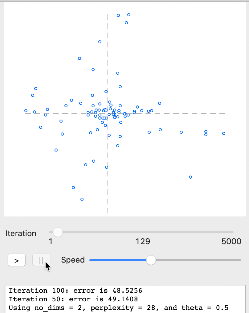
Figure 28: t-SNE results - animation stop at 129

As the iterations proceed further, the point cloud constantly changes until it starts to attain a more stable form. For example, in Figure 29, the plot is shown with the process stopped after 662 iterations. The error of 0.245 at iteration 650 is very similar to the result for a full set of 5000 iterations. Basically, after 650-700 iterations, the process has stabilized around a particular configuration with only minor changes.

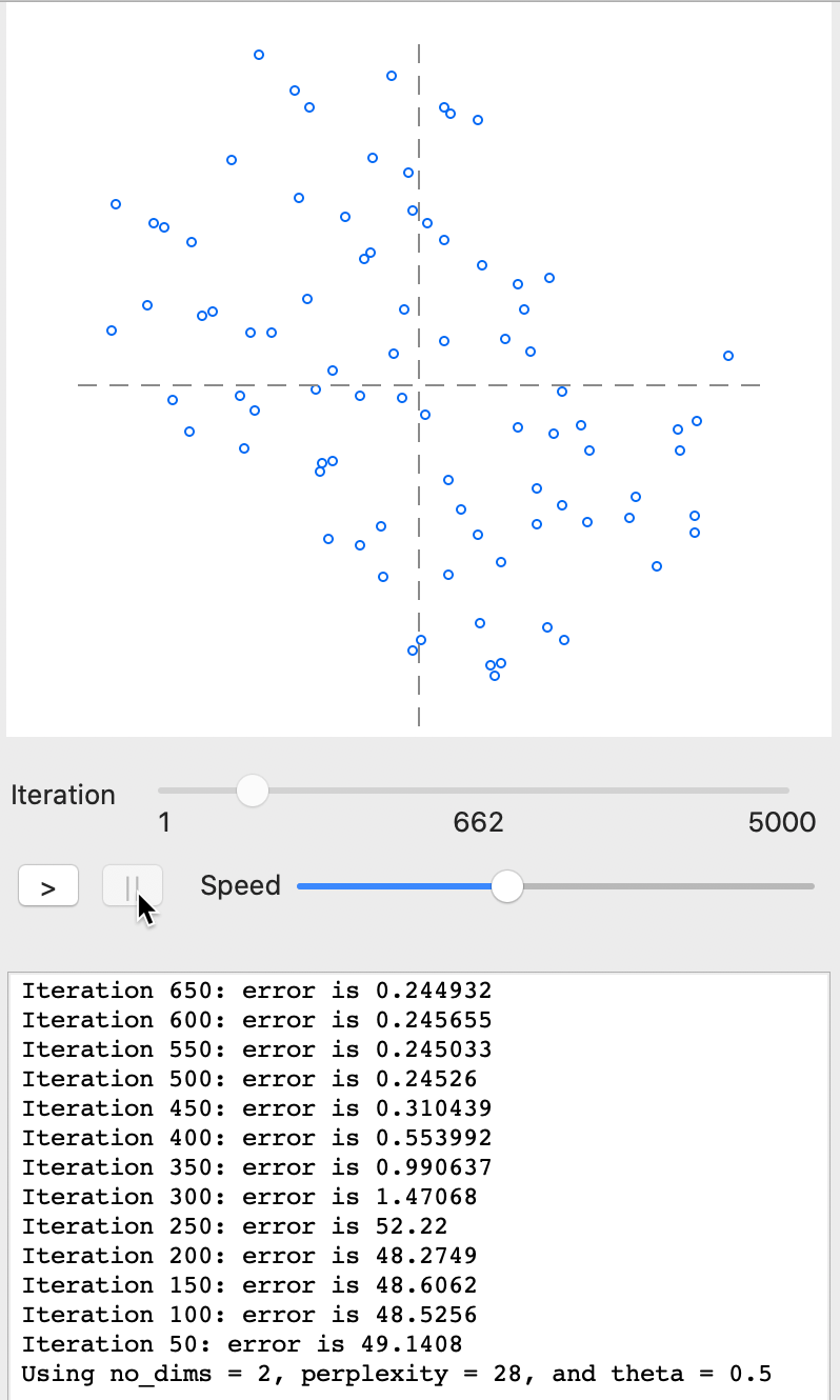
Figure 29: t-SNE results - animation stop at 662

The corresponding final scatter plot in Figure 30 shows a rank correlation of 0.726, the same as for the full set of iterations.

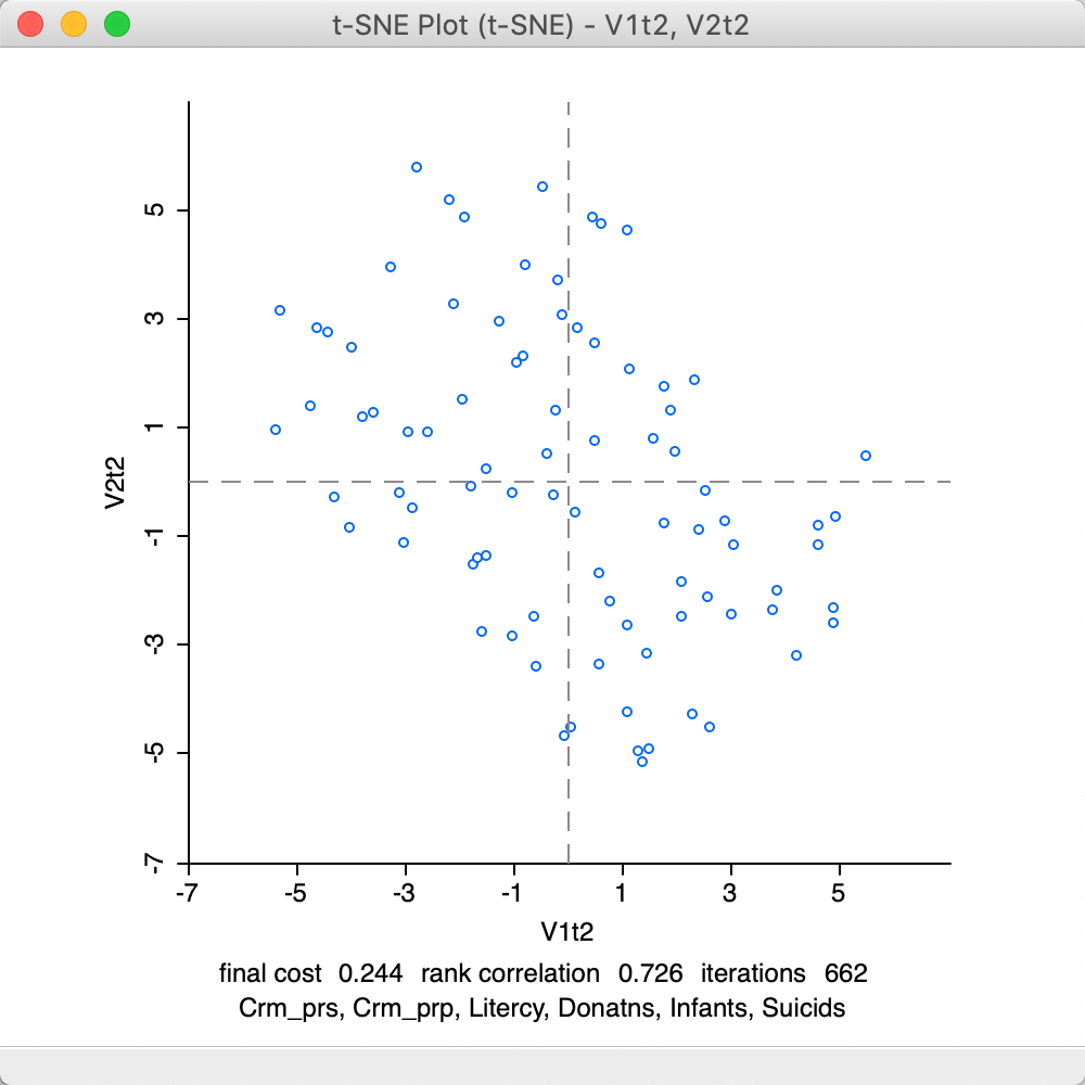
Figure 30: t-SNE result plot at 662

Categorical variable

The t-SNE interface includes the same option as MDS to visualize the position of data points that correspond to a particular category, as in Figure 20. However, for t-SNE, this does not only apply to the final scatter plot (similar to its MDS counterpart in Figure 21), but also during the iterations shown in the animation panel.

Using the same selection as for MDS, the iteration plot shows how the region categories move around as the process converges, e.g., as in Figure 31. Here as well, some more flexibility can be obtained through the use of the bubble chart, as illustrated below in the section on Visualizing a categorical variable.

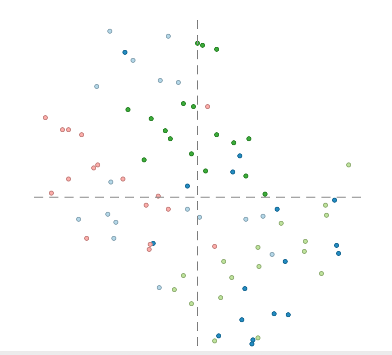
Figure 31: t-SNE iterations with categorical variables

Tuning the optimization

The number of options to tune the optimization algorithm may seem a bit overwhelming. However, in many instances, the default settings will be fine, although some experimenting is always a good idea.

To illustrate the effect of some of the parameters, we will change Theta, the Perplexity and the Iteration Switch for the Momentum (see the technical discussion for details on the meaning and interpretation).

The Barnes-Hut algorithm implemented for t-SNE sets the Theta parameter to 0.5 by default. This is the criterion that determines the extent of simplification for the \(q_{ij}\) measures in the gradient equation. This parameter is primarily intended to allow the algorithm to scale up to large data sets. In smaller data sets, like in our example, we may want to set this to zero, which avoids the simplification. The result is as in Figure 32. There are slight differences with the default result, but overall the performance is somewhat worse. The final cost is 0.312 (compared to 0.241) and the rank correlation is inferior as well, 0.682 relative to 0.726.

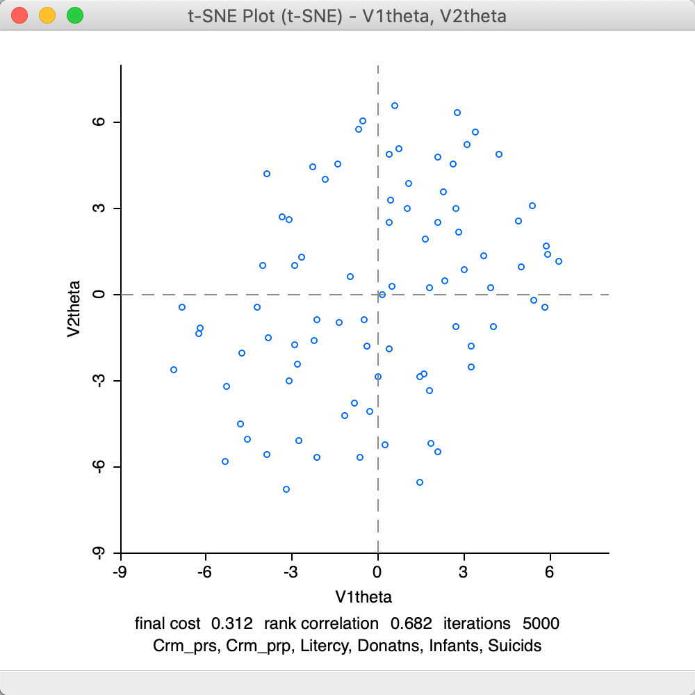
Figure 32: t-SNE result plot with theta = 0

The second parameter to adjust is the Perplexity (with Theta set back to its default value). This is a rough proxy for the number of neighbors and is by default set to its maximum (\(n/3 = 28\)). The results for a value of 15 are given in Figure 33. Again, the results are much worse than for the default setting, with a final cost of 0.449 and a rank correlation of 0.537.

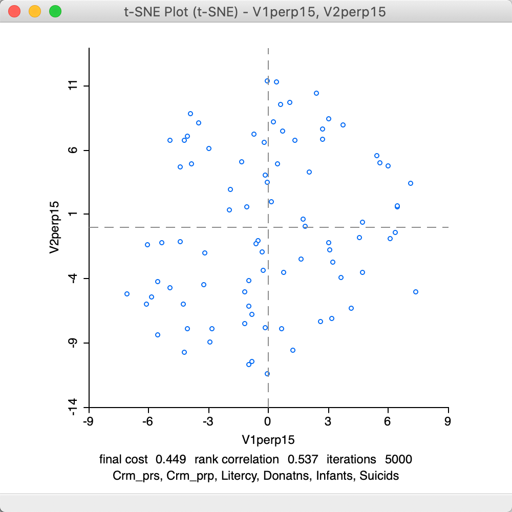
Figure 33: t-SNE result plot with perplexity = 15

The final adjustment is to the Iteration Switch for the Momentum parameter, which decides at which point in the iterations the Momentum moves from 0.5 to 0.8. The default value is 250. In Figure 34, the result is shown for a value of 100. Again, the results are worse than for the default settings, with a final cost of 0.293 and a rank correlation of 0.718.

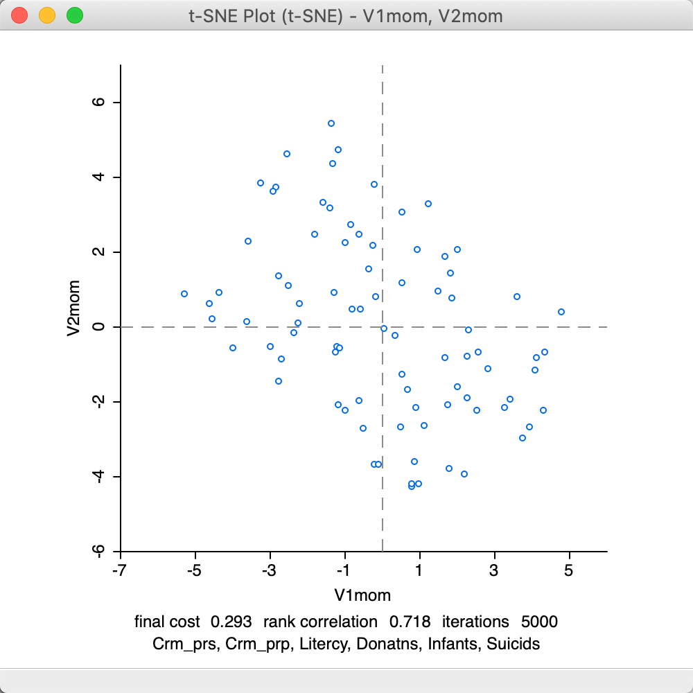
Figure 34: t-SNE result plot with momentum iteration switch=100

Further experimentation with the various parameters can provide deep insight into the dynamics of this complex algorithm, although the specifics will vary from case to case. Also, as argued in van der Maaten (2014), the default settings are an excellent starting point. .

Interpretation

The interpretation of the results of t-SNE is the same as for the standard MDS plots. Linking and brushing between subsets of points in the scatter plot and PCP graphs will provide insight into the particulars of the observation groupings.

As mentioned, a common interest is to assess the extent to which certain pre-specified clusters are reflected in the scatter plot, both for MDS as well as for t-SNE. This is visualized when a Category Variable is specified. In addition, a more flexible visualization of various categories (pre-defined groupings or clusters) can be obtained by leveraging the functionality of the bubble plot.

Visualizing a categorical variable

To illustrate this feature, we will use the Region variable in the Guerry data set. The pre-specified groupings or clusters should be represented by an integer unique value or categorical variable, but that is not the case for Region, which in the original data set is given by a letter code. A quick way to turn the letter code into a numerical value is to create a unique value map (as shown in the left-hand panel of Figure 36) and save the categories to a new variable, say regno.⁸ In addition, to get the bubble chart to work properly, we need a variable that is set to a constant.⁹

We invoke the chart by means of Explore > Bubble Chart from the menu, or from the Bubble Chart toolbar icon. In the interface, shown in Figure 35, we specify the first coordinate as X-Axis (here, V1tsne) and the second coordinate at Y-Axis (V2tsne). Next, we set the Bubble Size to the constant we just created, and Standard Deviation Color to regno.

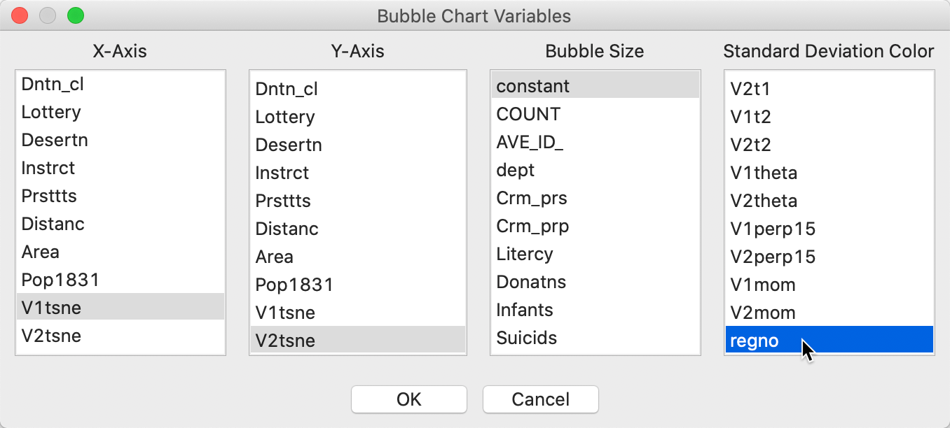
Figure 35: t-SNE bubble chart interface

The default bubble plot color is for a standard deviational classification, but we can change that by right clicking and setting Classification Themes > Unique Values. Finally, we use the Adjust Bubble Size option to change the size of the circles to something meaningful. The result is as in the right-hand panel of Figure 36.

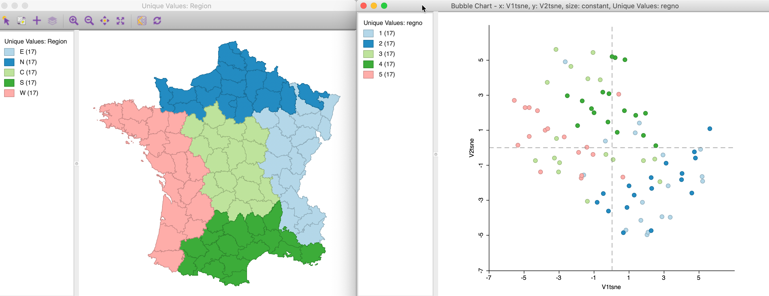
Figure 36: t-SNE points by region

The match between the locations in the t-SNE plot and the five main regions is far from perfect, although the locations in the north and east tend to group in the lower-right quadrant, whereas the south and central ones are more in the upper half of the chart. Nevertheless, this illustrates the mechanism through which different cluster or regional definitions can be mapped to the corresponding locations in a MDS scatter plot. We pursue this in more detail in the discussion of attribute and locational similarity that follows.

Attribute and Locational Similarity

The points in the MDS scatter plot can be viewed as locations in a two-dimensional attribute space. This is an example of the use of geographical concepts (location, distance) in contexts where the space is non-geographical. It also allows us to investigate and visualize the tension between attribute similarity and locational similarity, two core components underlying the notion of spatial autocorrelation. These two concepts are also central to the various clustering techniques that we consider in later chapters.

An explicit spatial perspective is introduced by linking the MDS scatter plot with various map views of the data. In addition, it is possible to exploit the location of the points in attribute space to construct spatial weights based on neighboring locations. These weights can then be compared to their geographical counterparts to discover overlap. Finally, we can construct an alternative version of the local neighbor match test using the distances in an MDS plot instead of the full k-nearest neighbor distances. We discuss each of these prespectives in turn. For further technical details, see Anselin and Li (2020).

Linking MDS scatter plot and map

To illustrate the extent to which neighbors in attribute space correspond to neighbors in geographic space, we link a selection of close points in the MDS scatter plot to a quartile map of the first principal component. Clearly, this can easily be extended to all kinds of maps of the variables involved, including co-location maps that pertain to multiple variables, cluster maps, etc.

In Figure 37, we selected nine points that are close in attribute space in the right-hand panel of an MDS scatter plot using the classic metric approach for our six variables. We connect this to a quartile map of the first principal component (using the default SVD setting), and assess the extent to which the locations match. All points in the graph are in the upper quartile for PC1, and many, but not all, are also closely located in geographic space. We can explore this further by brushing the scatter plot to systematically evaluate the extent of the match between attribute and locational similarity for any number of variables. In addition, we can apply this principle to a link between locations in any of the univariate or multivariate cluster maps and the MDS scatter plot.

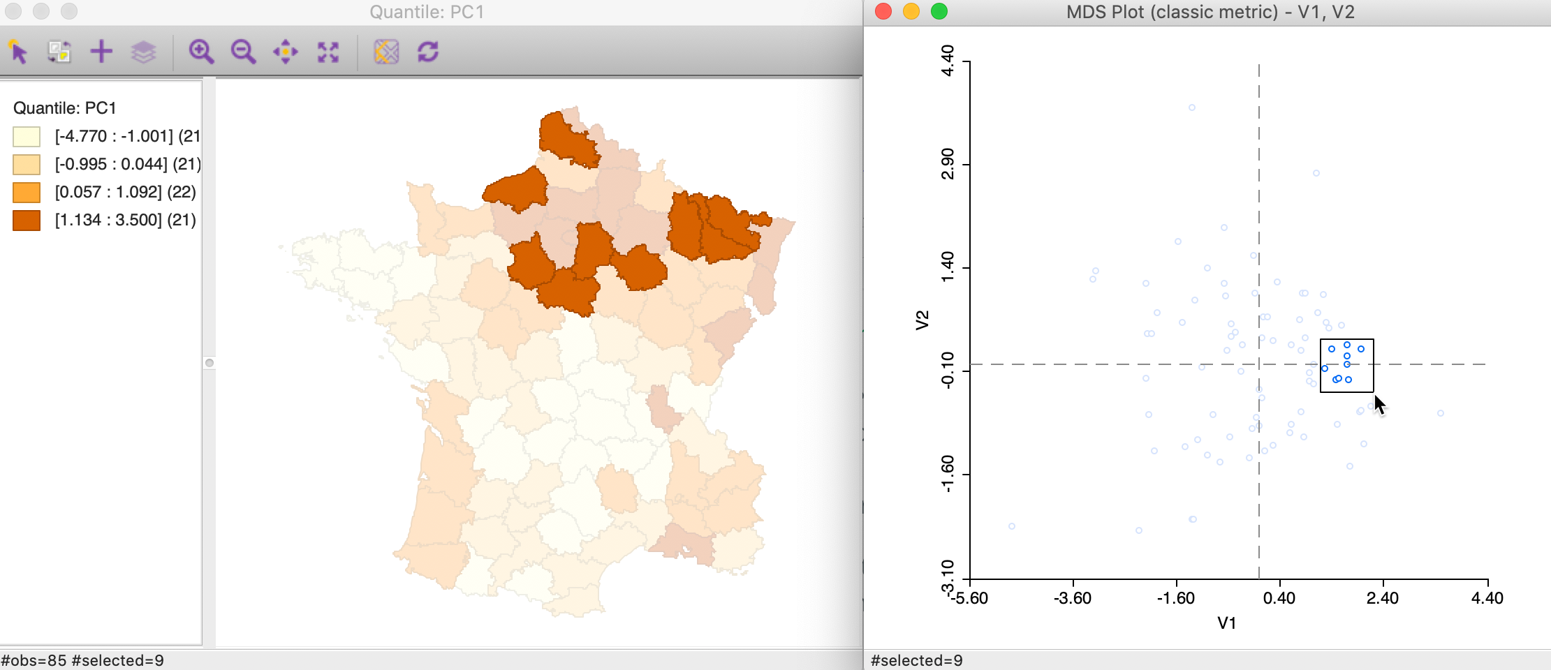
Figure 37: Neighbors in MDS space

Alternatively, we can brush the map and identify the matching observations in the MDS scatter plot, as in Figure 38. This reverses the logic and assesses the extent to which neighbors in geographic space are also neighbors in attribute space. In this instance in our example, the result is mixed, with some evidence of a match between the two concepts for selected points, but not for others.

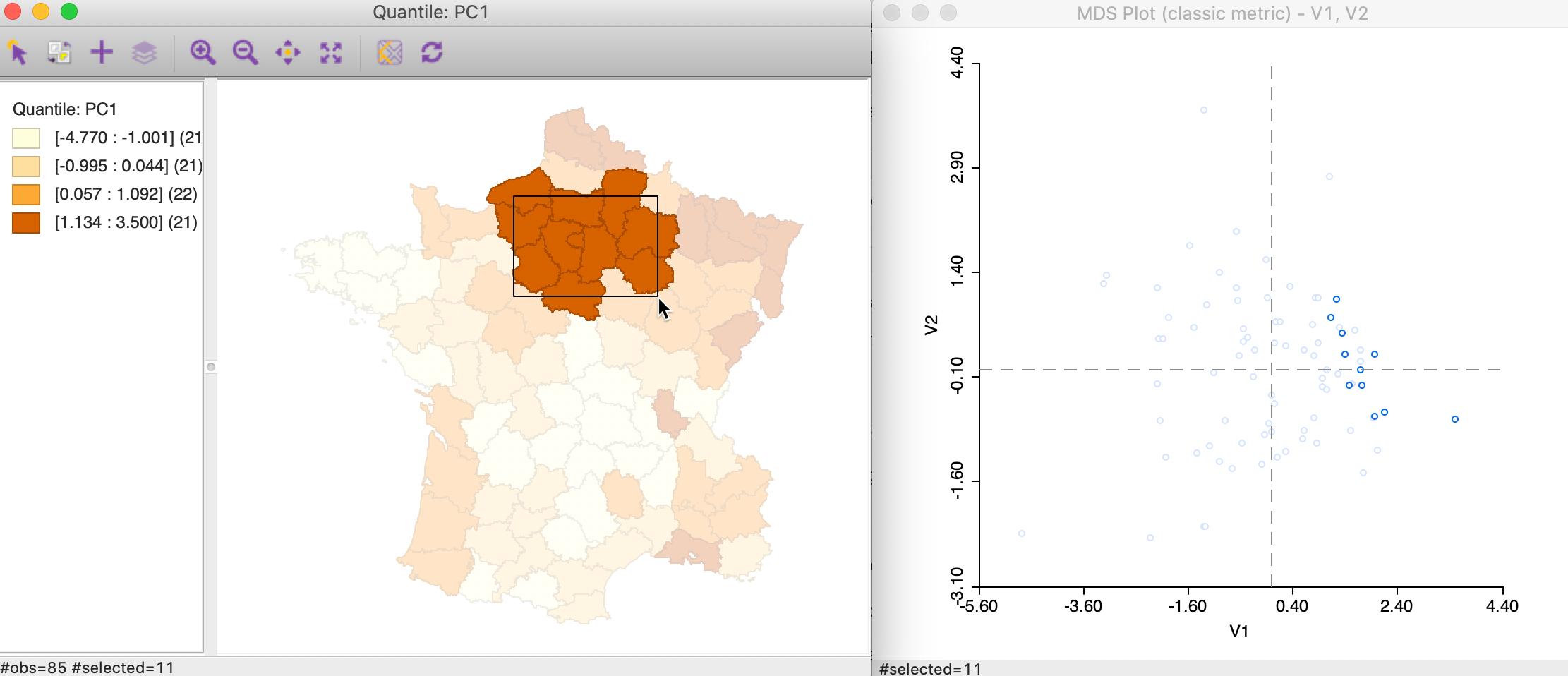
Figure 38: Brushing the map and MDS

With an active spatial weights matrix, we can explore this more precisely by using the Connectivity > Show Selection and Neighbors in the map. This will highlight the corresponding points in the MDS scatter plot.

Spatial weights from MDS scatter plot

The points in the MDS scatter plot can be viewed as locations in an embedded attribute space. As such, they can be mapped. In such a point map, the neighbor structure among the points can be exploited to create spatial weights, in exactly the same way as for geographic points (e.g., distance bands, k-nearest neighbors, contiguity from Thiessen polygons). Conceptually, such spatial weights are similar to the distance weights created from multiple variables, but they are based on inter-observation distances from an embedded high-dimensional object in two dimensions. While this involves some loss of information, the associated two-dimensional visualization is highly intuitive.

In GeoDa, there are three ways to create spatial weights from points in a MDS scatter plot. One is to explicitly create a point layer using the MDS coordinates (for example, V1 and V2), by means of Tools > Shape > Points from Table. Once the point layer is in place, the standard spatial weights functionality can be invoked.

A second way pertains only to distance weights. It again uses the Weights Manager, but with the Variables option for Distance Weight. For example, in Figure 39, this is illustrated for k-nearest neighbor weights with \(k = 6\) and the t-SNE coordinates as the variables. Since these coordinates are already normalized in a way, we can safely use the Raw setting for standardization.

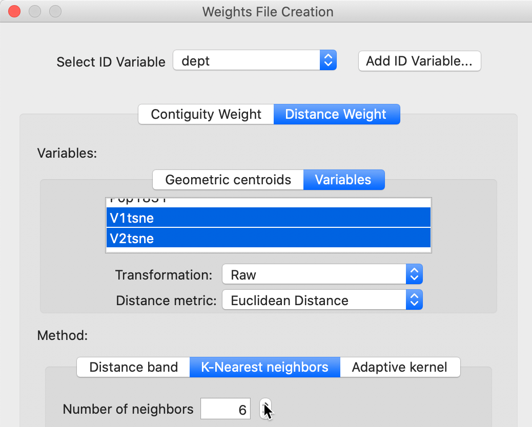
Figure 39: Create weights using MDS coordinates

A final method applies directly to the MDS scatterplot. As shown in Figure 40, one of the options available is to Create Weights.

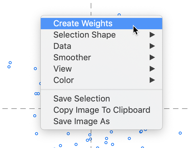
Figure 40: Create weights from MDS scatter plot

This brings up the standard Weights File Creation interface, as shown in Figure 41. The example again illustrates k-nearest neighbor weights with \(k=6\). The difference with the previous approach is that the MDS coordinates do not need to be specified, but are taken directly from the MDS scatter plot where the option is invoked. In addition, it is also possible to create contiguity weights from the Thiessen polygons associated with the scatter plot points.

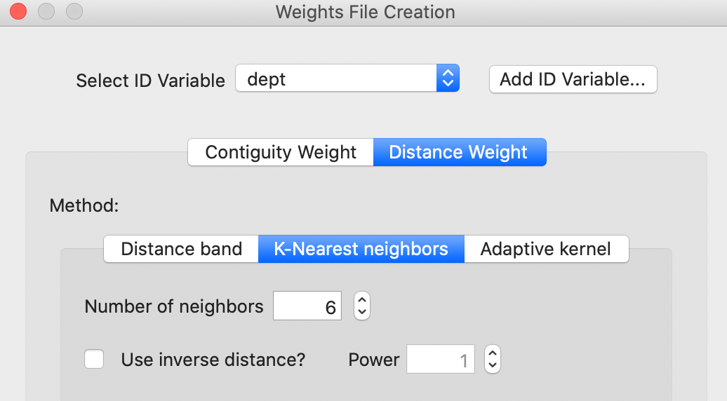
Figure 41: Queen weights from MDS scatter plot

Once created, the weights file appears in the Weights Manager and its properties are listed, in the same way as for other weights.

Matching attribute and geographic neighbors

We can now investigate the extent to which the k-nearest neighbors in geographic space match neighbors in attribute space using the Intersection functionality in the Weights Manager (Figure 42).

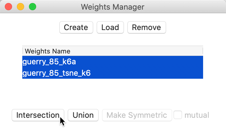
Figure 42: Intersection knn weights

This creates a gal weights file that lists for each observation the neighbors that are shared between the two k-nearest neighbor files. As is to be expected, the resulting file is much sparser than the original weights. In the Histogram, we can see the distribution of the number of matches. We can then Save Connectivity to Table to create a variable that reflects this cardinality. Such a variable then lends itself to a Unique Values Map, as in Figure 43. Even though the associated colors are not ideal (they can easily be changed), this identifies five departments that have four out of the six nearest neighbors in common between the two weights.

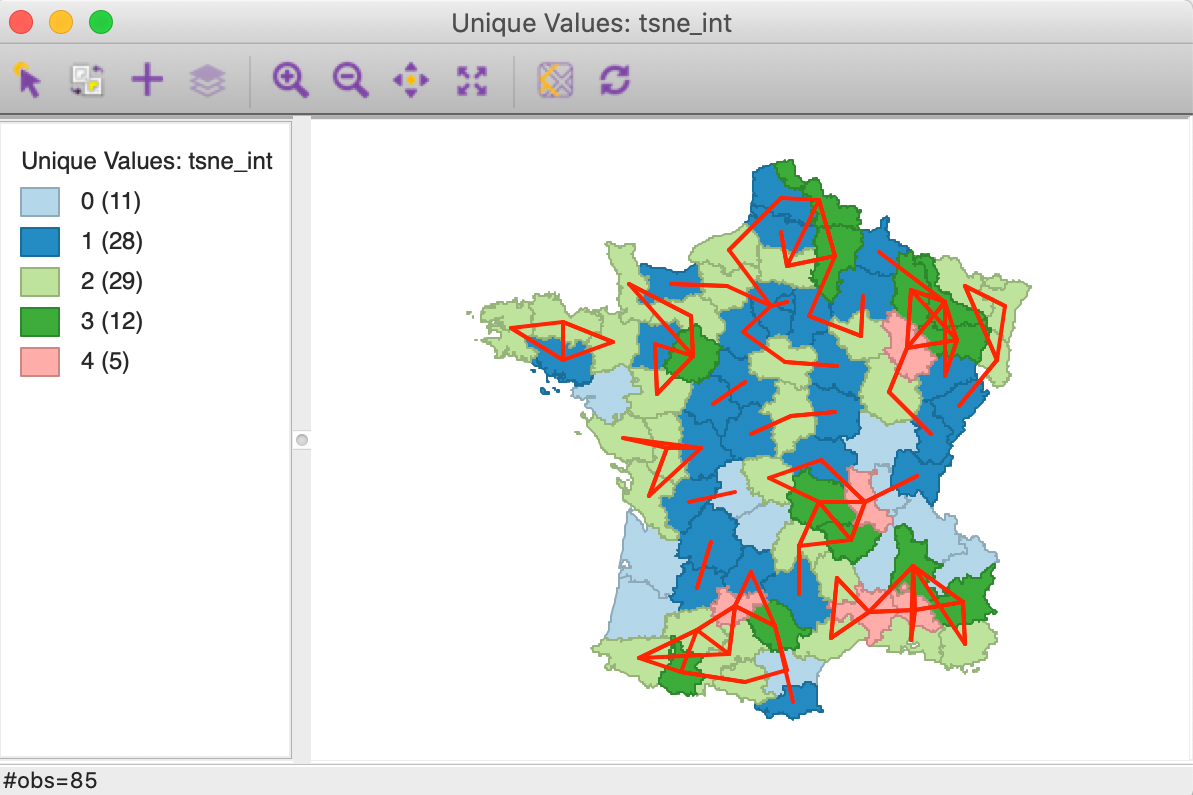
Figure 43: Intersection knn weights for geography and MDS t-SNE

When the connectivity graph is superimposed on the map, the location of the overlap becomes very clear. The red lines on the map correspond with matches between the two types of k-nearest neighbors.

The presence of several sets of interconnected vertices suggest the presence of multivariate clustering, albeit without a measure of significance. The local neighbor match test is based on the same principle, but also provides a measure of significance (as well as a better colored unique values map).

Comparing the neighbor structure of different scaling algorithms

We can use the Intersection functionality for spatial weights to compare the nearest neighbor structures implied by classic metric MDS, SMACOF and t-SNE in terms of how closely they match the geographical nearest neighbor relations. We just illustrated the use of the connectivity graph and the neighbor cardinality to visualize the similarity between two types of weights. In addition, we can also interpret the summary characteristics in the Weights Manager to get an assessment of the degree of agreement.

For example, we compare the percentage non-zero to the standard result, which is 7.06% for k=6 in our example. For the classic metric MDS weights, this percentage is 1.59%, for SMACOF it is 1.72% and for t-SNE 1.97%. Compared to the maximum achievable, the relevant percentages are 22.5% for MDS, 24.4% for SMACOF and 27.9% for t-SNE. We call this metric the common coverage percentage. The results confirm the superiority of t-SNE in terms of capturing local structure, relative to the two MDS methods, which are more geared towards respecting large distances.

We can also compare the common coverage percentage between the three scaling algorithms: for metric MDS-SMACOF this is 55.2%, for MDS-t-SNE 41.5%, and for SMACOF-t-SNE 45.6%. This further highlights that t-SNE captures a different type of neighbor relation than the classic MDS methods. The specific locations of overlap can be explored further using the connectivity graph as shown above.

Local neighbor match test based on MDS neighbors

A final, more formal approach to check the similarity between neighbors in attribute space and neighbors in geographic space is as a special case of the local neighbor match test. Instead of using the k-nearest neighbor relation for the high-dimensional space, we can use the same relation in the two- or three-dimensional MDS space.

In the interface for Space > Local Neighbor Match Test, we select the MDS coordinates as the variables. For example, in Figure 44, the t-SNE coordinates are selected to create k-nearest neighbor weights for \(k=6\).

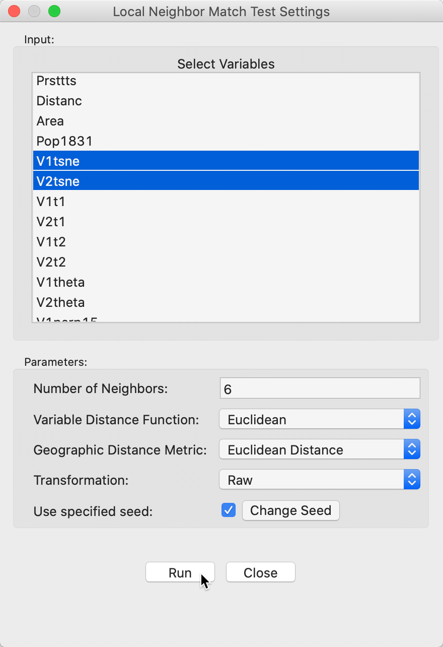
Figure 44: K-nearest neigbhors weights of t-SNE coordinates

Clicking on Run gives the option to save the cardinality of the weights intersection between the attribute knn weights and the geographical knn weights, as well as the associated probability of finding that many neighbors in common. Next, the associated unique value map is brought up that shows the cardinalities of the match for each location, with the corresponding connectivity graph superimposed, as in Figure 45. Note that this is identical to the map shown in Figure 43, except for the different colors.

The cpval column in the data table reveals that locations with four matches have an associated \(p\)-value of 0.00011. This map can then be compared to the results found for the multi-attribute k-nearest distances.¹⁰

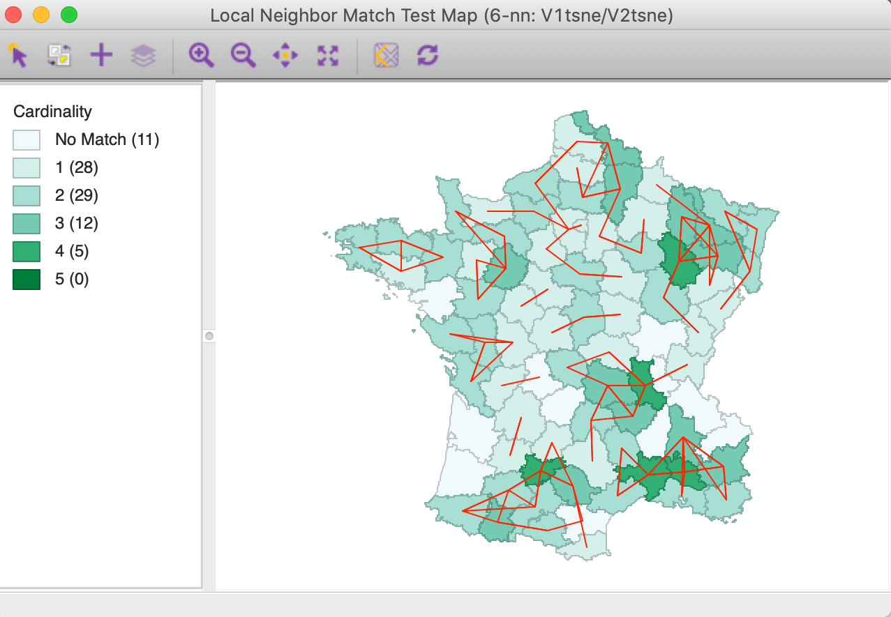
Figure 45: Local neighbor match test for t-SNE coordinates

Appendix

Connection between a squared distance matrix and the Gram matrix

The reason why the solution to the metric MDS problem can be found in a fairly straightforward analytic way has to do with the interesting relationship between the squared distance matrix and the Gram matrix for the observations, the matrix \(XX'\). Note that this only holds for Euclidean distances. As a result, the Manhattan distance option is not available for the classic metric MDS.

The squared Euclidean distance between two points \(i\) and \(j\) in \(k\)-dimensional space is: \[d^2_{ij} = \sum_{h=1}^k (x_{ih} - x_{jh})^2,\] where \(x_{ih}\) corresponds to the \(h\)-th value in the \(i\)-th row of \(X\) (i.e., the \(i\)-th observation), and \(x_{jh}\) is the same for the \(j\)-th row. After working out the individual terms of the squared difference, this becomes: \[d^2_{ij} = \sum_{h=1}^k (x_{ih}^2 + x_{jh}^2 - 2 x_{ih}x_{jh}).\] The full matrix \(D^2\) for all pairwise distances between observations for a given variable (column) \(h\) simply contains the corresponding term in each position \(i-j\). For the diagonal terms, this boils down to \(x_{ih}^2 + x_{ih}^2 - 2 x_{ih}x_{ih} = 0\), as desired. Each off-diagonal element is \(x_{ih}^2 + x_{jh}^2 - 2 x_{ih}x_{jh}\). The full matrix \(D\) for a given variable/column \(h\) can be expressed as the sum of three matrices. The first matrix has \(x_{ih}^2\) in each row \(i\) (so \(x_{1h}^2\) in the first row, \(x_{2h}^2\) in the second row, etc.). The second matrix has \(x_{ih}^2\) in each column \(i\) (so \(x_{1h}^2\) in the first column, \(x_{2h}^2\) in the second column, etc.). The third matrix has all the cross-products, or \(x_hx_h'\). Note that the diagonal of the matrix \(x_h x_h'\) is made up of the squares, \(x_{ih}^2\). So, with this diagonal expressed as a vector \(c_h\), it turns out that the squared distance matrix between all pairs of observations for a given variable \(h\) is: \[D^2_h = c_{h} \iota' + \iota c_{h}' - 2 x_{h} x_{h}',\] where \(\iota\) is a \(n \times 1\) vector of ones.¹¹ As a result, the full \(n \times n\) squared distance matrix consists of the sum of the individual squared distance matrices over all variables/columns: \[D^2 = c \iota' + \iota c' - 2 XX',\] since \(\sum_{h = 1}^k x_h x_h' = XX'\), and with each element of \(c = \sum_{h=1}^k x_{ih}^2\), for \(i = 1, \dots, n\).

Double centering the squared distance matrix

An important result in metric MDS is that the Gram matrix can be obtained from \(D^2\) by double centering: \[XX' = - \frac{1}{2} (I - M)D^2(I - M),\] where \((I - M)\) is as above. With some tedious matrix algebra, we can show that this actually holds. Since \(X\) is standardized, \(X' \iota = 0\) and \(\iota' X = 0\) (the sum of deviations from the mean is zero). Also, \(\iota ' \iota = n\).

First, we post-multiply \(D^2\) by \((I - M)\). This yields: \[c \iota' + \iota c' - 2 XX' - (1/n) c \iota' \iota \iota' - (1/n) \iota c' \iota \iota' - (2/n) XX'\iota \iota',\] Recall that \(c\) contains the diagonal elements of \(XX'\) so that \(c ' \iota\) is the sum of the diagonal elements, or the trace of \(XX'\), say \(t\), a scalar. Moreover, with a standardized matrix \(X\) as we use here, \(t = n\) (since the variance for each variable equals 1), although in the end, that does not matter to obtain the correct result. Using the other properties from above, the expression becomes: \[c \iota' + \iota c' - 2 XX' - (n/n) c \iota' - (t/n) \iota \iota' - 0 = \iota c' - 2 XX' - (t/n) \iota \iota'.\] Now, pre-multiplying this by \((I - M)\) gives: \[ \iota c' - 2 XX' - (t/n) \iota \iota' - (1/n) \iota \iota' \iota c' + (2/n) \iota \iota' XX' + (t/n^2) \iota \iota' \iota \iota',\] or, again using the trace property: \[\iota c' - 2 XX' - (t/n) \iota \iota' - (n/n) \iota c' + 0 + (t/n) \iota \iota',\] and removing the terms that cancel out: \[ - 2 XX',\] the desired result.

Finding coordinates from the Gram matrix

While we have established the equivalence between a doubly-centered squared distance matrix and the matrix \(XX'\), that does not give us coordinates for \(X\) that would yield he proper distances. Assuming that we only have \(XX'\), what would such coordinates be?

Here, we resort again to the eigenvalue decomposition of \(XX'\), which is a square and symmetric \(n \times n\) matrix. The decomposition is: \[XX' = VGV',\] with the all matrices of dimension \(n \times n\), \(G\) a diagonal matrix with the eigenvalues on the diagonal, and \(V\) a matrix with the eigenvectors as the columns. Since the matrix is symmetric, all the eigenvalues are positive, so that their square roots exist. We can thus write the decomposition as: \[XX' = VG^{1/2}G^{1/2}V' = (VG^{1/2})(VG^{1/2})'.\] In other words, the matrix \(VG^{1/2}\) can play the role of \(X\). It is not the same as \(X\), in fact it is expressed as coordinates in a different (rotated) axis system, but they yield the same distances, so they have the same relative positions. In practice, to express this in lower dimensions, we only select the first and second (and sometimes third) columns of \(VG^{1/2}\), so we only need the two/three largest eigenvalues and corresponding eigenvectors. They can be readily computed by means of the power iteration method.

Power iteration method to obtain eigenvalues/eigenvectors

The power method is an iterative approach to obtain the eigenvector associated with the largest eigenvalue of a matrix \(A\). It is found from an iteration that starts with an arbitrary unit vector, say \(x_0\),¹² and iterates by applying higher and higher powers to the transformation \(x_{k} = A x_{k-1} = A^k x_{0}\). So, starting with an arbitrary unit initial vector \(x_0\), we get \(x_1 = Ax_0\), and then subsequently \(x_2 = Ax_1 = A^2x_0\), and so on until convergence (i.e., the difference between \(x_k\) and \(x_{k-1}\) is less than a pre-defined threshold). The end value, say \(x_k\), is a good approximation to the dominant eigenvector of \(A\).¹³

The associated eigenvalue is found from the so-called Rayleigh quotient: \[\lambda = \frac{x_k' A x_k}{x_k ' x_k}.\] The second largest eigenvector is found by applying the same procedure to the matrix \(B\): \[B = A - \lambda x_k x_k',\] using the largest eigenvalue and eigenvector just computed. The idea can be applied to obtain more eigenvalues/eigenvectors, although typically this method is only used to compute a few of the largest ones. The procedure can also be applied to the inverse matrix \(A^{-1}\) to obtain the smallest eigenvalues.

Iterative majorization of the stress function

The discussion here is largely based on the materials in Borg and Groenen (2005), Chapter 8, except that the notation is slightly different, to keep it consistent with the rest of the notes.

The objective of the iterative majorization of the stress function is to find a simpler function that bounds the stress function from above (so, the stress function is always smaller), and to iterate until its minimum and the minimum of the stress function coincide.

The first step in this is to turn the stress function into a matrix expression, as a function of the solution matrix \(Z\). It consists of the three parts given in the main text: \[S(Z) = \sum_{i<j} \delta_{ij}^2 + \sum_{i<j} d_{ij}^2(Z) - 2 \sum_{i<j} \delta_{ij}d_{ij}(Z)\] One way to write the difference between observation pairs \(i-j\) for coordinate \(h\) in \(Z\) (i.e., the values contained in column \(h\)), or \(z_{ih}- z_{jh}\), is by considering an \(n \times 1\) vector \(e_i\) to pick out element \(i\) and a vector \(e_j\) to pick out element \(j\). These vectors are respectively the \(i-th\) and \(j-th\) column of an identity matrix. Then, \((e_i - e_j)'z_{*h}\) yields a \(1 \times n\) vector with \(z_{ih} - z_{jh}\). To obstain the squared distance between \(i\) and \(j\) for a given variable/column \(h\) we thus use \(z_{*h}'(e_i - e_j)(e_i - e_j)'z_{*h}\). In the MDS literature, the matrix \((e_i - e_j)(e_i - e_j)' = A_{ij}\), a \(n \times n\) matrix with \(a_{ii} = a_{jj} = 1\) and \(a_{ij} = a_{ji} = -1\). Considering all column dimensions of \(Z\) jointly then gives the squared distance between \(i\) and \(j\) as \(d^2_{ij}(Z) = \sum_{h=1}^k z_h'A_{ij}z_h = tr Z'A_{ij}Z\), with \(tr\) as the trace operator. Summing this over all the pairs (without double counting) gives \[\sum_{i<j} d_{ij}^2(Z) = tr(Z' \sum_{i <j}A_{ij}Z) = tr(Z'VZ),\] with the \(n \times n\) matrix \(V = \sum_{i <j}A_{ij}\), a row and column centered marix (i.e., each row and each column sums to zero), with \(n - 1\) on the diagonals and \(-1\) in all other positions. Given the row and column centering, this matrix is singular.

The third term, \(- 2 \sum_{i<j} \delta_{ij}d_{ij}(Z)\) is where the majorization comes into play. Consider a new set of coordinates, \(Y\), which will be critical in setting up the majorization function. The “trick” is to take advantage of the so-called Cauchy-Schwarz inequality: \[ \sum_m z_my_m \leq (\sum_m z_m^2)^{1/2} (\sum_m y_m^2)^{1/2},\] i.e., the sum of the cross-products of all values \(m\) of \(z\) and \(y\) is less or equal to the product of the norms for each of the variables (the square root of the sums of squares, a measure of length for a vector).

If we take \(z\) as \((z_i - z_j)\) and \(y\) as \((y_i - y_j)\), for the \(i\)-th and \(j\)-th rows of respectively \(Z\) and \(Y\), with \(i \neq j\), then we have: \[ \sum_m (z_{im} - z_{jm})(y_{im} - y_{jm}) \leq [\sum_m (z_{im} - z_{jm})^2]^{1/2}[\sum_m (y_{im} - y_{jm})^2]^{1/2},\] where the right hand side corresponds to \(d_{ij}(Z).d_{ij}(Y)\), i.e., the product of the distance between \(i\) and \(j\) for \(Z\) and \(Y\). For \(z = y\), equality results, but in all other instances the right hand side dominates the left-hand side. After moving around some terms, we end up with: \[ - d_{ij}(Z) \leq - \frac{\sum_m (z_{im} - z_{jm})(y_{im} - y_{jm})}{d_{ij}(Y)}.\] Using the same expression for \(A_{ij}\) as above, this can also be written as: \[- d_{ij}(Z) \leq - tr(Z'A_{ij}Y) / d_{ij}(Y),\] or: \[- d_{ij}(Z) \leq - tr[Z'(A_{ij}/d_{ij}(Y))Y],\] since \(d_{ij}(Y)\) is just a scalar. Extending this logic, we obtain: \[- \delta_{ij} d_{ij}(Z) \leq - tr[Z'(\delta_{ij}/d_{ij}(Y))A_{ij}Y],\] where \(\delta_{ij}/d_{ij}(Y)\) is just a scalar multiple of the four non-zero entries in \(A_{ij}\), based on the distance between \(i\) and \(j\) computed for the elements of \(Y\).

We now get the counterpart of the matrix \(V\) above from summing the \(A_{ij}\) over all the relevant pairs, each multiplied by \(\delta_{ij}/d_{ij}(Y)\). Note that this ratio ends up in positions \(i,i\) and \(j,j\), and its negative in \(i,j\) and \(j,i\). Consequently: \[\sum_{i < j} (\delta_{ij}/d_{ij}(Y))A_{ij} = B(Y),\] with off-diagonal elements \(B_{ij} = - \delta_{ij} / d_{ij}(Y)\), and diagonal elements \(B_{ii} = - \sum_{j, j\neq i} B_{ij}\).

The majorization condition for the third term can then be written as: \[ - tr[Z'B(Z)Z] \leq - tr[Z'B(Y)Y].\]

The majorization of the complete stress function follows as: \[ S(Z) = \sum_{i<j} \delta_{ij}^2 + tr(Z'VZ) - 2tr[Z'B(Z)Z] \leq \sum_{i<j} \delta_{ij}^2 + tr(Z'VZ) - 2tr[Z'B(Y)Y].\] It is minimized with respect to \(Z\) for \(2VZ - 2B(Y)Y = 0\).¹⁴

As it turns out, \(V\) is singular (due to the double centering), so that the usual solution \(Z = V^{-1}B(Y)Y\) doesn’t work. Instead, we have to resort to a generalized or Moore-Penrose inverse \(V^+\). For double-centered matrices, this takes the special form \(V^+ = (V + \iota \iota')^{-1} - n^{-2} \iota \iota'\), with \(\iota\) as a vector of ones.¹⁵ The second term doesn’t matter, since \(\iota'B(Y) = 0\), due to the double centering. For the case we consider, where we do not use weights, the first term simplifies to \(V^+ = (1/n)(I - (1/n)\iota \iota')\) so that the solution becomes: \[Z = (1/n) B(Y)Y,\] the so-called Guttman transform.

In the GeoDa implementation of SMACOF, the initial values for each column of \(Y\) are set as standard normal random variates (using the default seed set in the global Preferences).

Barnes-Hut optimization of t-SNE

The implementation of t-SNE in GeoDa is adopted from the tree-based algorithms outlined in van der Maaten (2014), themselves based on a principle proposed by Barnes and Hut (1986), hence the reference to Barnes-Hut optimization. The van der Maaten approach is based on two simplifications that allow the algorithms to scale to very large data sets. One strategy is to parse the distribution \(P\) and eliminate all the probabilities \(p_{ij}\) that are too small in some sense. The other strategy is to do something similar to the probabilities \(q_{ij}\) in the sense that the value for several individual points that are close together is represented by a central point (hence reducing the number of individual \(q_{ij}\) that need to be evaluated). This is the Barnes-Hut aspect.

The t-SNE gradient is separated into two parts (in the same notation as before): \[\frac{\partial C}{\partial z_i} = 4 [\sum_{j \neq i} p_{ij}q_{ij}U(z_i - z_j) - \sum_{j \neq i} q_{ij}^2 U (z_i - z_j)],\] where the first part (the cross-products) represents an attractive force and the second part (the squared probabilities) represents a repulsive force. The simplification of the \(p_{ij}\) targets the first part (converting many products to a value of zero), the simplification of \(q_{ij}\) addresses the second part (reducing the number of expressions that need to be evaluated).

In order to simplify the \(p_{ij}\) we consider those pairs that are more than \(3u\) apart (where \(u\) is the perplexity, i.e., roughly the target number of neighbors). For the points \(j\) that are farther away than this critical distance, the probability \(p_{ij}\) is set to zero. The rationale for this is that the value of \(p_{ij}\) for those pairs that do not meet the closeness criterion is likely to be very small and hence can be ignored (i.e., their \(p_{ij}\) is set to \(0\)). As a result of the choice of the distance criterion, the value for perplexity set as an option can be at most \(n/3\).¹⁶ The parsing of \(p_{ij}\) is implemented by means of a so-called vantage-point tree (VP tree). In essence, this tree divides the space into those points that are closer than a given distance to a reference point (the vantage-point) and those that are further away. By applying this recursively, the data get partitioned into smaller and smaller entities such that neighbors in the tree are likely to be neighbors in space (see Yianilos 1993 for technical details). The VP tree is used to carry out a nearest neighbor search so that all \(j\) that are not in the nearest neighbor set for a given \(i\) result in \(p_{ij} = 0\). Note that the \(p_{ij}\) do not change during the optimization, since they pertain to the high-dimensional space, so this calculation only needs to be done once.

The Barnes-Hut algorithm deals with the layout of the points \(z\) at each iteration. First, a quadtree is created for the current layout.¹⁷ The tree is traversed (depth-first) and at each node a decision is made whether the points in that cell can be effectively represented by their center. The logic behind this is that the distance from \(i\) to all the points \(j\) in the cell will be very similar, so rather than computing each individual \(q_{ij}^2U(z_i - z_j)\) for all the \(j\) in the cell, they are replaced by \(n_c q^2_{ic}(1 + ||z_i - z_c ||^2)^{-1} (z_i - z_c)\), where \(n_c\) is the number of points in the cell and \(z_c\) are the coordinates of a central (representative) point. The denser the points are in a given cell, the greater the computational gain.¹⁸

A critical decision is the selection of those cells for which the simplification is appropriate. This is set by the \(\theta\) parameter to the optimization program (Theta in Figure 25), such that: \[\frac{r_c}{||z_i - z_c||} < \theta,\] where \(r_c\) is the length of the diagonal of the cell square. In other words, the cell is summarized when the diagonal of the cell is less than \(\theta\) times the distance between a point \(i\) and the center of the cell. With \(\theta\) set to zero, there is no simplification going on and all the \(q_{ij}\) are computed at each iteration.

The software implementation of this algorithm in GeoDa is based on the C++ code by van der Maaten.

References

Anselin, Luc, and Xun Li. 2020. “Tobler’s Law in a Multivariate World.” Geographical Analysis. https://doi.org/10.111/gean.12237.

Banerjee, Sudipto, and Anindya Roy. 2014. Linear Algebra and Matrix Analysis for Statistics. Boca Raton: Chapman & Hall/CRC.

Barnes, J., and P. Hut. 1986. “A Hierarchical O(N log N) Force-Calculation Algorithm.” Nature 324 (4): 446–49.

Borg, Ingwer, and Patrick J.F. Groenen. 2005. Modern Multidimensional Scaling, Theory and Applications (2nd Ed). New York, NY: Springer.

de Leeuw, Jan. 1977. “Applications of Convex Analysis to Multidimensional Scaling.” In Recent Developments in Statistics, edited by J.R. Barra, F. Brodeau, G. Romier, and B. van Cutsem, 133–45. Amsterdam: North Holland.

de Leeuw, Jan, and Patrick Mair. 2009. “Multidimensional Scaling Using Majorization: SMACOF in R.” Journal of Statistical Software 21 (3).

Hinton, Geoffrey E., and Sam T. Roweis. 2003. “Stochastic Neighbor Embedding.” In Advances in Neural Information Processing Systems 15 (NIPS 2002), edited by S. Becker, S. Thun, and K. Obermayer, 833–40. Vancouver, BC: NIPS.

Kruskal, Joseph. 1964. “Multidimensional Scaling by Optimizing Goodness of Fit to a Non-Metric Hypothesis.” Psychometrika 29: 1–17.

Lee, John A., and Michel Verleysen. 2007. Nonlinear Dimensionality Reduction. New York, NY: Springer-Verlag.

Mead, A. 1992. “Review of the Development of Multidimensional Scaling Methods.” Journal of the Royal Statistical Society. Series D (the Statistician) 41: 27–39.

Rao, C., and S.Mitra. 1971. Generalized Inverse of a Matrix and Its Applications. New York, NY: John Wiley.

Shepard, Roger N. 1962a. “The Analysis of Proximities: Multidimensional Scaling with an Unknown Distance Function I.” Psychometrika 27: 125–40.

———. 1962b. “The Analysis of Proximities: Multidimensional Scaling with an Unknown Distance Function II.” Psychometrika 27: 219–46.

Torgerson, Warren S. 1952. “Multidimensional Scaling, I: Theory and Method.” Psychometrika 17: 401–19.

———. 1958. Theory and Methods of Scaling. New York, NY: John Wiley.

van der Maaten, Laurens. 2014. “Accelerating t-SNE Using Tree-Based Algorithms.” Journal of Machine Learning Research 15: 1–21.

van der Maaten, Laurens, and Geoffrey Hinton. 2008. “Visualizing Data Using t-SNE.” Journal of Machine Learning Research 9: 2579–2605.

Wattenberg, Martin, Fernanda Viégas, and Ian Johnson. 2016. “How to Use t-SNE Effectively.” Distill. https://doi.org/10.23915/distill.00002.

Yianilos, Peter N. 1993. “Data Structures and Algorithms for Nearest Neighbor Search in General Metric Spaces.” In Proceedings of the ACM-SIAM Symposium on Discrete Algorithms, 311–21. Philadelphia, PA: SIAM.

---

1. University of Chicago, Center for Spatial Data Science – anselin@uchicago.edu↩

2. For an extensive discussion, see Borg and Groenen (2005), Chapter 8. A software implementation is outlined in de Leeuw and Mair (2009).↩

3. In a more general exposition, as in Borg and Groenen (2005) and de Leeuw and Mair (2009), the distances can be weighted, primarily to deal with missing values, but we will ignore that aspect here.↩

4. To find the actual values (not reported separately in GeoDa), a routine such as the eigen function in R can be employed. However, keep in mind that the signs of the elements of the eigenvector may differ between routines. In the illustration given here, the actual values used by GeoDa for the default setting are reported.↩

5. Unlike what is the case for the 2D MDS scatter plot, the statistics can currently not be turned off in 3D.↩

6. For technical details related to the so-called crowding problem, see the discussion in van der Maaten and Hinton (2008).↩

7. Due to the Barnes-Hut approximation, the final cost value does not equal the value for the error at the last iteration. As mentioned in the discussion of the Barnes-Hut optimization of t-SNE, when Theta is not zero, several values of \(q_{ij}\) are replaced by the center of the corresponding quadtree block. The final cost reported is computed with the values for all \(i-j\) pairs included in the calculation, and does not use the simplified \(q_{ij}\), whereas the error reported for each iteration uses the simplified version.↩

8. The specific steps involved are invoked by selecting Classification Themes > Unique Values and choosing Region as the variable. Then Save Categories will save integer values to a new variable.↩

9. To accomplish this, we use the Calculator with the Univariate > Assign option and set the constant to 1, as an integer (the actual value doesn’t matter, since we will be adjusting the size of the bubble).↩

10. See Anselin and Li (2020) for further examples.↩

11. Post-multiplying the vector \(c\) with a row vector of ones puts the same element in each row, pre-multiplying its transpose by a column vector of ones puts the same element in each column.↩

12. \(x_0\) is typically a vector of ones divided by the square root of the dimension. So, if the dimension is \(n\), the value would be \(1/\sqrt{n}\).↩

13. For a formal proof, see, e.g., Banerjee and Roy (2014), pp. 353-354.↩

14. This exploits some results from matrix partial derivatives, namely that \(\partial Z'VZ / \partial Z = VZ\) and \(\partial Z'BY / \partial Z = BY\).↩

15. The formal result is based on Rao and S.Mitra (1971), pp. 181-182.↩

16. In van der Maaten and Hinton (2008) a range for perplexity between 5 and 50 was suggested, but in smaller data sets, this is not possible under the Barnes-Hut approach. For example, in the Guerry example, with \(n=85\), the maximum value for perplexity would be \(85/3 = 28\), which is much less than 50.↩

17. A quadtree is a tree data structure that recursively partitions the space into squares as long as there are points in the resulting space. For example, the bounding box of the points is first divided into four squares. If one of those is empty, that becomes an endpoint in the tree (a leaf). For those squares with points in them, the process is repeated, again stopping whenever a square is empty. This structure allows for very fast searching of the tree. In three diminsions, the counterpart (using cubes) is called an octree.↩

18. For further technical details, see van der Maaten (2014).↩

GeoDa is maintained by lixun910. This page was generated by GitHub Pages using the Cayman theme by Jason Long.