Spatial Clustering (2)

Spatially Constrained Clustering - Hierarchical Methods

Introduction

We now move our focus to methods that impose contiguity as a hard constraint in a clustering procedure. Such methods are known under a number of different terms, including zonation, districting, regionalization, spatially constrained clustering, and the p-region problem. They are concerned with dividing an original set of n spatial units into p internally connected regions that maximize within similarity (for recent reviews, see, e.g., Murray and Grubesic 2002; Duque, Ramos, and Suriñach 2007; Duque, Church, and Middleton 2011).

In the previous chapter, we covered approaches that impose a soft constraint, in the form of a trade-off between attribute similarity and spatial similarity. In the methods considered in the current and next chapter, the contiguity is a strict constraint, in that clusters can only consist of entities that are geographically connected. As a result, in some cases the resulting attribute similarity may be of poor quality, when dissimilar units are grouped together primarily due to the contiguity constraint.

We consider three sets of methods. We start by introducing spatial constraints into an agglomerative hierarchical clustering procedure, following the approach reviewed in Murtagh (1985) and Gordon (1996), among others. Next, we outline two common algorithms, i.e., SKATER (Assunção et al. 2006) and REDCAP (Guo 2008; Guo and Wang 2011). SKATER stands for Spatial `K’luster Analysis by Tree Edge Removal, and obtains regionalization through a graph partitioning approach. REDCAP stands for REgionalization with Dynamically Constrained Agglomerative clustering and Partitioning, and consists of a family of six hierarchical regionalization methods.

As before, the methods considered here share many of the same options with previously discussed techniques as implemented in GeoDa. Common options will not be considered, but the focus will be on aspects that are specific to the spatial perspective.

To illustrate these methods, we continue to use the Guerry data set.

Objectives

• Understand how imposing spatial constraints affects hierarchical agglomerative clustering

• Understand the tree partioning method underlying the SKATER algorithm

• Identify contiguous clusters by means of the SKATER algorithm

• Understand the connection between SCHC, SKATER and the REDCAP family of methods

• Identify contiguous clusters by means of the REDCAP algorithm

GeoDa functions covered

• Clusters > SCHC
• Clusters > skater
  • set minimum bound variable
  • set minimum cluster size
• Clusters > redcap

Preliminaries

We continue to use the Guerry data set and also need a spatial weights matrix in the form of queen contiguity.

Spatially Constrained Hierarchical Clustering (SCHC)

Principle

Spatially constrained hierarchical clustering is a special form of constrained clustering, where the constraint is based on contiguity (common borders). We have earlier seen how a minimum size constraint can be imposed on classic clustering algorithms. The spatial constraint is more complex in that it directly affects the way in which elemental units can be merged into larger entities.

The idea of including contiguity constraints into agglomerative hierarchical clustering goes back a long time, with early overviews of the principles involved in Lankford (1969), Murtagh (1985) and Gordon (1996). Recent software implementations can be found in Guo (2009) and Recchia (2010).

The clustering logic is identical to that of unconstrained hierarchical clustering, and the same expressions are used for linkage and updating formulas, i.e., single linkage, complete linkage, average linkage, and Ward’s method (we refer to the relevant chapter for details). The only difference is that now a contiguity constraint is imposed.

More specifically, two entities \(i\) and \(j\) are merged when the dissimilarity measure \(d_{ij}\) is the smallest among all pairs of entities, subject to \(w_{ij} = 1\) (i.e., a non-zero spatial weight). In other words, merger is only carried out when the corresponding entry in the spatial weights (contiguity) matrix is non-zero. Another way to phrase this is that the minimum of the dissimilarity measure is only searched for those pairs of observations that are contiguous.

As before, the dissimilarity measure is updated for the newly merged unit using the appropriate formula. In addition, the weights matrix needs to be updated to reflect the contiguity structure of the newly merged units.

Consider this more closely. In the first step, the weights matrix is of dimension \(n \times n\). If observations \(i\) and \(j\) are merged into a new entity, say \(A\), then the resulting matrix will be of dimension \((n - 1) \times (n-1)\) and the two original rows/columns for \(i\) and \(j\) will be replaced by a new row/column for \(A\). For the new matrix, the row elements \(w_{Ah} = 1\) if either \(w_{ih} = 1\) or \(w_{jh} = 1\) (or both are non-zero), and similarly for the column elements.

The next step thus consists of a new dissimilarity matrix and new contiguity matrix, both of dimension \((n - 1) \times (n-1)\). At this point the process repeats itself. As for other hierarchical clustering methods, the end result is a single cluster that contains all the observations. The process of merging consecutive entities is graphically represented in an dendrogram, as before. A fully worked example is included in the Appendix.

One potential complication is so-called inversion, when the dissimilarity criterion for the newly merged unit with respect to remaining observations is better than for the merged units themselves. This link reversal occurs when \(d_{i \cup j, k} \lt d_{ij}\). It is only avoided in the complete linkage case (for details, see Murtagh 1985; Gordon 1996). This problem is primarily one of interpretation and does not preclude the clustering methods from being applied.

Implementation

Spatially constrained hierarchical clustering is invoked as the first item in the corresponding group in the list associated with the Clusters item on the toolbar, as in Figure 1, or from the menu, as Clusters > SCHC.

Figure 1: SCHC cluster option

Ward’s linkage

The menu brings up the usual cluster variable interface with the same general structure as for the unconstrained hierarchical clustering. The variable selection is carried out in the left-hand panel of Figure 2. We choose the same six variables as before, Crm_prs, Crm_prp, Litercy, Donatns, Infants and Suicids. We use the variables in z-standardized form. In addition, we need to select a Spatial Weight, here set to queen contiguity in the guerry_85_q file. The default methods is Ward’s-linkage. As before, we also set the variable to which to save the cluster indicator, here CLw.

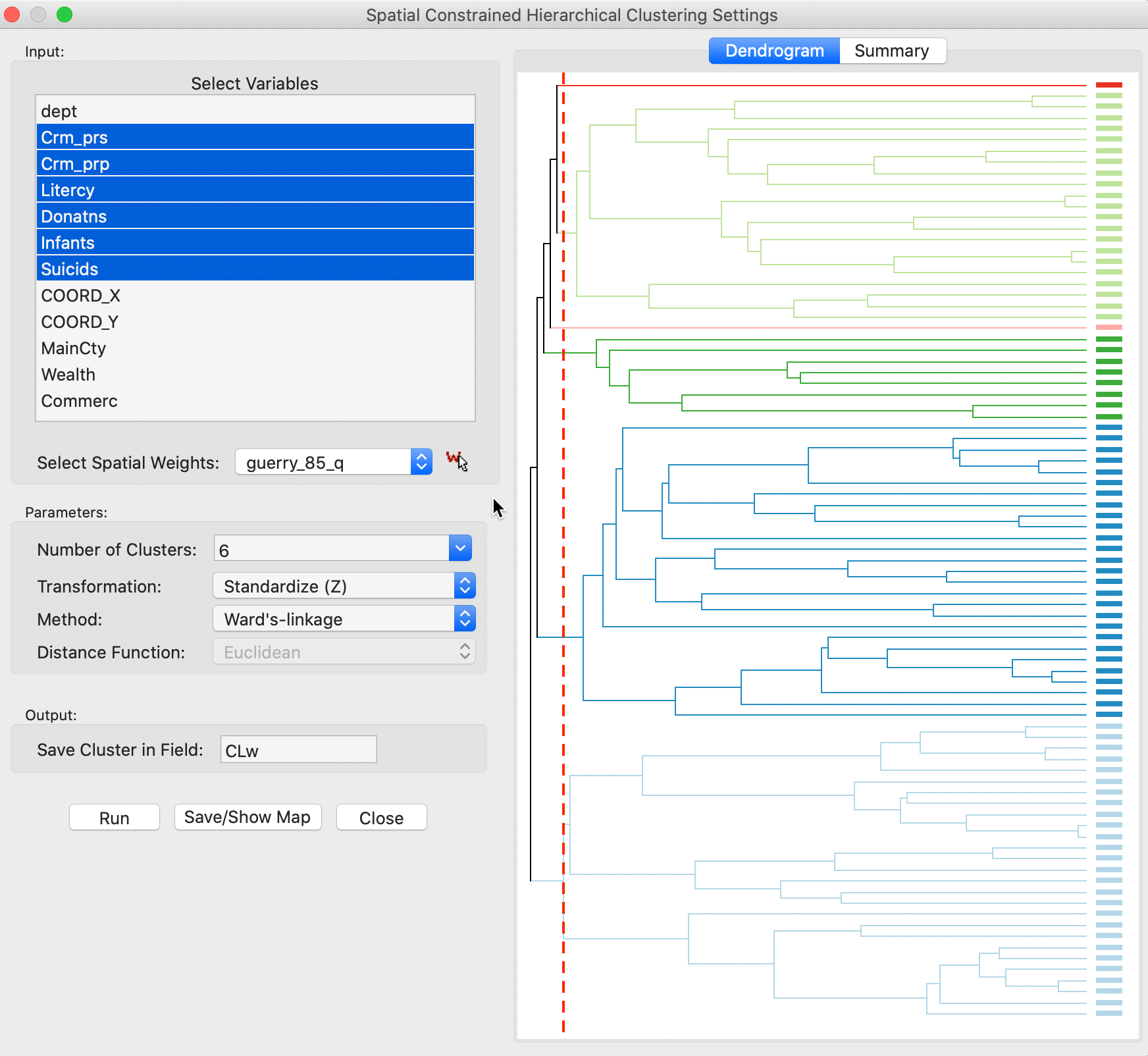
Figure 2: SCHC variable selection and initial run

The algorithm proceeds in two steps. Note that the Number of Clusters initially is set to 2, which we change to 6. Clicking on Run generates the dendrogram, shown in the right-hand panel of Figure 2. We can move the cut line (dashed red line) in the dendrogram to the desired number of clusters if it is different from the Number of Clusters in the interface. At this point, selecting Save/Show Map generates the cluster map shown in Figure 3.

We notice two well-balanced clusters of 27 departments, one with 21, one smaller one with 8 observations, and two singletons. As required, all clusters consist of contiguous spatial units.

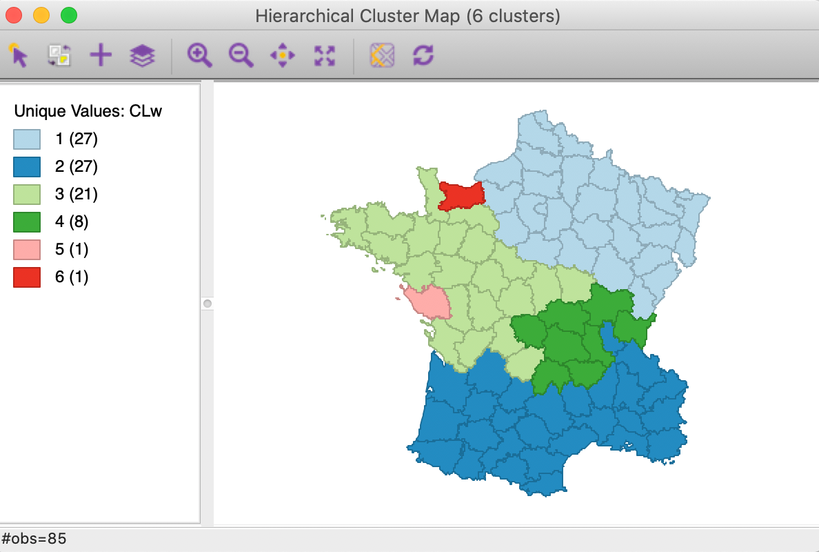
Figure 3: SCHC Ward method cluster map, k=6

The Summary button in the right-hand panel of Figure 2 brings up the usual summary characteristics, shown in Figure 4. The usual descriptors provide the cluster centers (in the original units), the within-cluster sum of squares for each cluster as well as the overall within and between cluster sum or squares. The ratio of between to total sum of squares amounts to 0.461812.

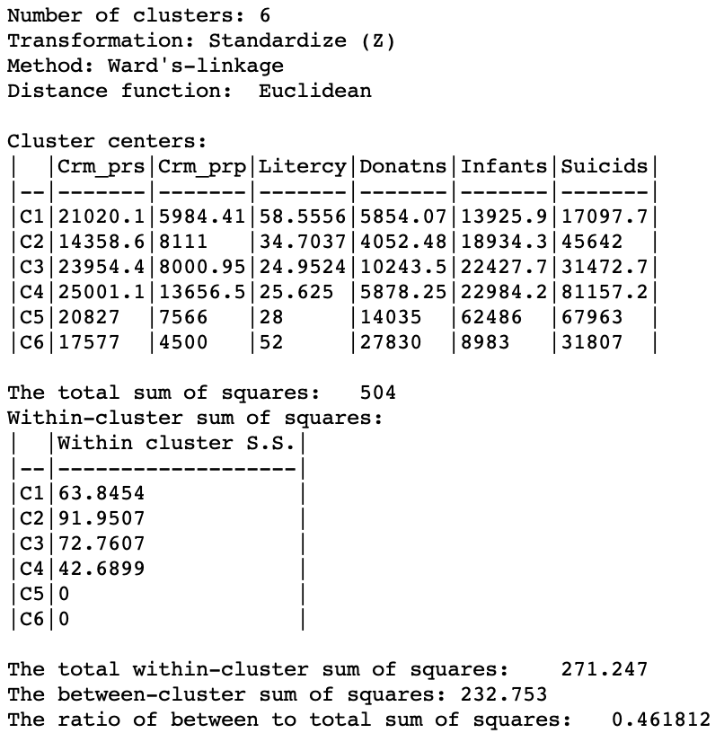
Figure 4: SCHC Ward method cluster characteristics, k=6

In order to put this into perspective, we show the results of the unconstrained hierarchical clustering routine with Ward’s linkage in Figure 5. The spatial pattern is quite different, with the larger clusters from Figure 3 split into the elements of several smaller clusters. There are no singletons, and the clusters range from 4 to 25 spatial units. Because the algorithm is unconstrained, the results for the ratio of between to total sum of squares is much better, at 0.532476. The difference with the constrained version gives a measure of the price to pay in order to achieve contiguity.

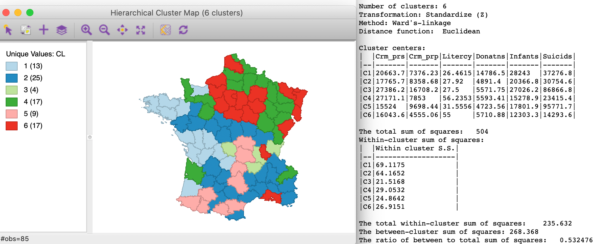
Figure 5: Ward method unconstrained hierarchical clustering, k=6

Single linkage

As in the unconstrained case, the Ward linkage methods is the default because it tends to yield compact clusters. As we saw earlier, the other linkage tend to result in a lot of unbalanced clusters and yield several singletons. The same is the case in the spatially constrained algorithms.

For completeness sake, we provide the results for the other three linkage methods, single linkage first.

The cluster map and summary characteristics for single linkage are shown in Figure 6. We obtain one large cluster with 80 observations and five singletons. The between to total ratio is 0.236071. These results are pretty dismal relative to the Ward linkage method.

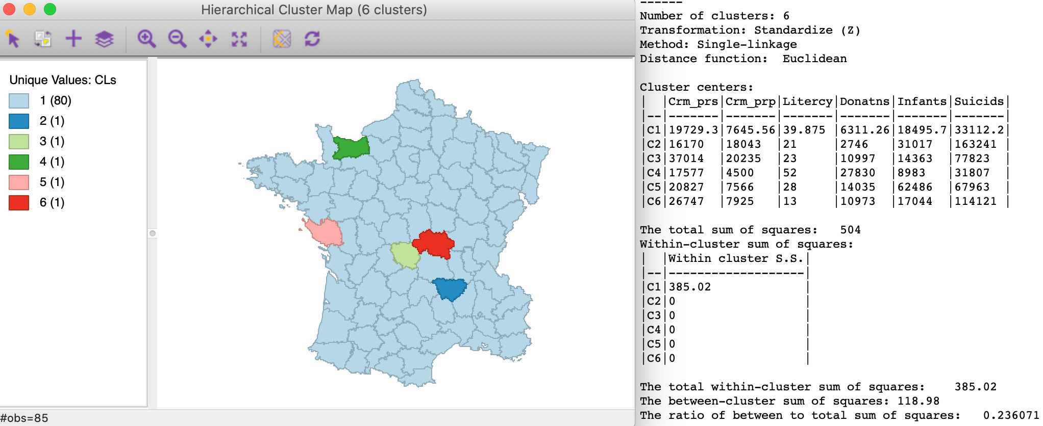
Figure 6: SCHC single linkage clustering, k=6

Complete linkage

As shown in Figure 7, the results for complete linkage are slightly better, with three non-singleton clusters and between to total ratio of 0.306119.

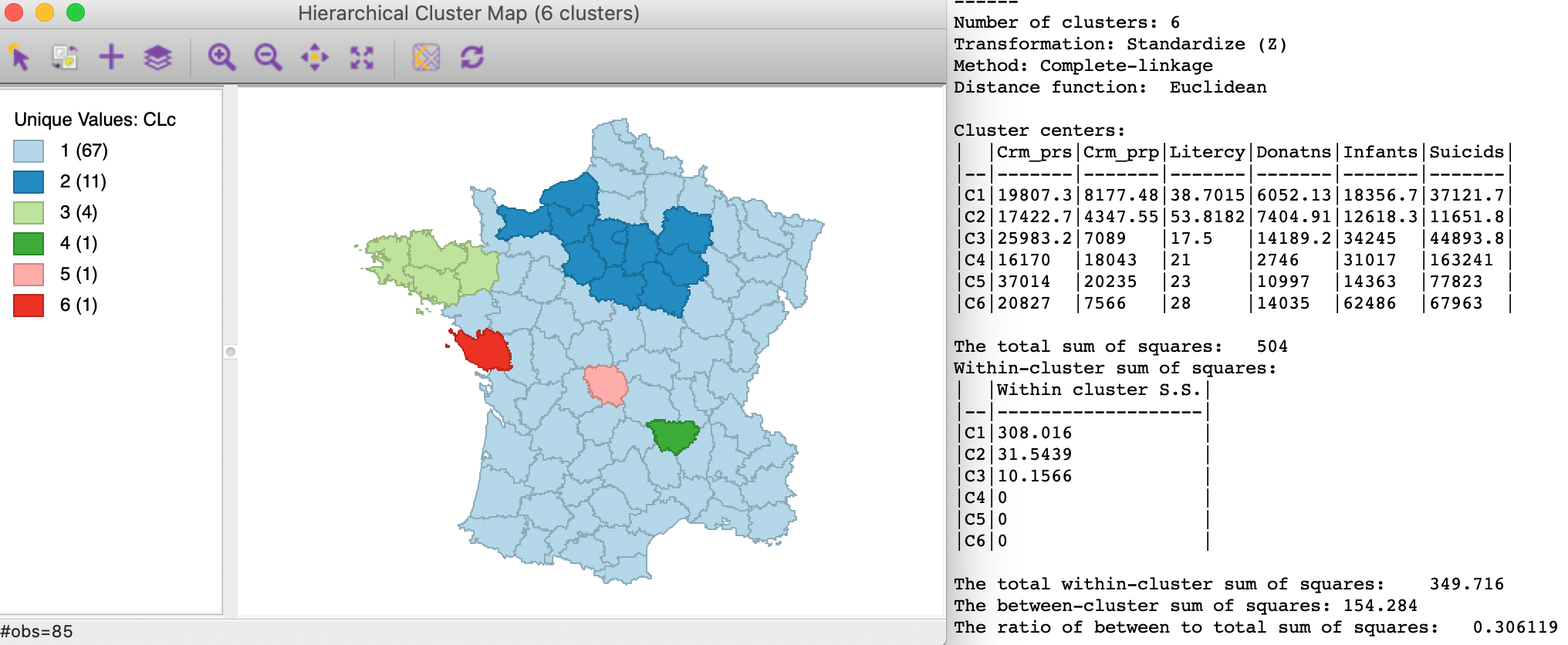
Figure 7: SCHC complete linkage clustering, k=6

Average linkage

Finally, average linkage, shown in Figure 8, again yields five singleton clusters, with a low between to total ratio of 0.246467, only slightly better than single linkage.

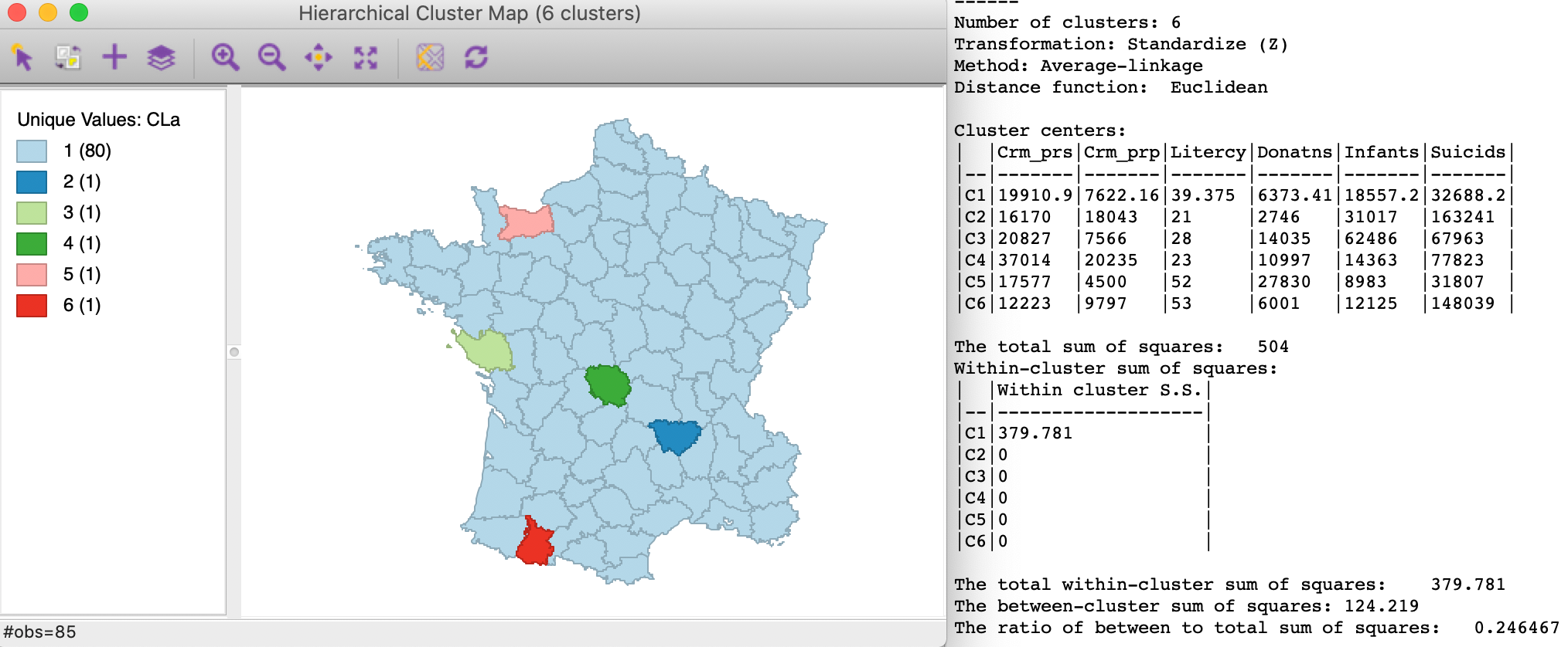
Figure 8: SCHC average linkage clustering, k=6

SKATER

Principle

The SKATER algorithm introduced by Assunção et al. (2006) is based on the optimal pruning of a minimum spanning tree that reflects the contiguity structure among the observations.²

The point of departure is a dissimilarity matrix that only contains weights for contiguous observations. In other words, we consider the distance \(d_{ij}\) between \(i\) and \(j\), but only for those pairs where \(w_{ij} = 1\) (contiguous). This matrix is represented as a graph with the observations as nodes and the contiguity relations as edges.

The full graph is reduced to a minimum spanning tree (MST), i.e., such that there is a path that connects all observations (nodes), but each is only visited once. In other words, the n nodes are connected by n-1 edges, such that the overall between-node dissimilarity is minimized. This yields a starting sum of squared deviations or SSD as \(\sum_i (x_i - \bar{x})^2\), where \(\bar{x}\) is the overall mean.

The objective is to reduce the overall SSD by maximizing the between SSD, or, alternatively, minimizing the sum of within SSD. The MST is pruned by selecting the edge whose removal increases the objective function (between group dissimilarity) the most. To accomplish this, each potential split is evaluated in terms of its contribution to the objective function.

More precisely, for each tree T, we consider \(\mbox{SSD}_T - (\mbox{SSD}_a + \mbox{SSD}_b)\), where \(\mbox{SSD}_a, \mbox{SSD}_b\) are the contributions of each subtree. The contribution is computed by first calculating the average for that subtree and then obtaining the sum of squared deviations.³ We select the cut in the subtree where the difference \(\mbox{SSD}_T - (\mbox{SSD}_a + \mbox{SSD}_b)\) is the largest.⁴

At this point, we repeat the process for the new set of subtrees to select an optimal cut. We continue until we have reached the desired number of clusters (k). A fully worked out example is given in the Appendix.

Like SCHC, this is a hierarchical clustering method, but here the approach is divisive instead of agglomerative. In other words, it starts with a single cluster, and finds the optimal split into subclusters until the value of k is satisfied. Because of this hierarchical nature, once the tree is cut at one point, all subsequent cuts are limited to the resulting subtrees. In other words, once an observation ends up in a pruned branch of the tree, it cannot switch back to a previous branch. This is sometimes viewed as a limitation of this algorithm.

In addition, the contiguity constraint is based on the original configurations and does not take into account new neighbor relations that follow from the combination of different observations into clusters, as was the case for SCHC.

Implementation

In GeoDa, the SKATER algorithm is invoked as the second item in the hierarchical group on the Clusters toolbar icon (Figure 1), or from the main menu as Clusters > skater.

Selecting this option brings up the Skater Settings dialog, shown in Figure 9. This interface has essentially the same structure as in all other clustering approaches. The panel provides a way to select the variables, the number of clusters and different options to determine the clusters. As for SCHC, we again have a Weights drop down list, where the contiguity weights must be specified. The SKATER algorithm does not work without a spatial weights file.

The Distance Function and Transformation options work in the same manner as for classic clustering. At the bottom of the dialog, we specify the Field or variable name where the classification will be saved. We consider the Minimum Bound and Min Region Size options below.

We continue with the Guerry example data set and select the same six variables as before: Crm_prs, Crm_prp, Litercy, Donatns, Infants, and Suicids. The spatial weights are based on queen contiguity (guerry_85_q). We initially set the number of clusters to 4.

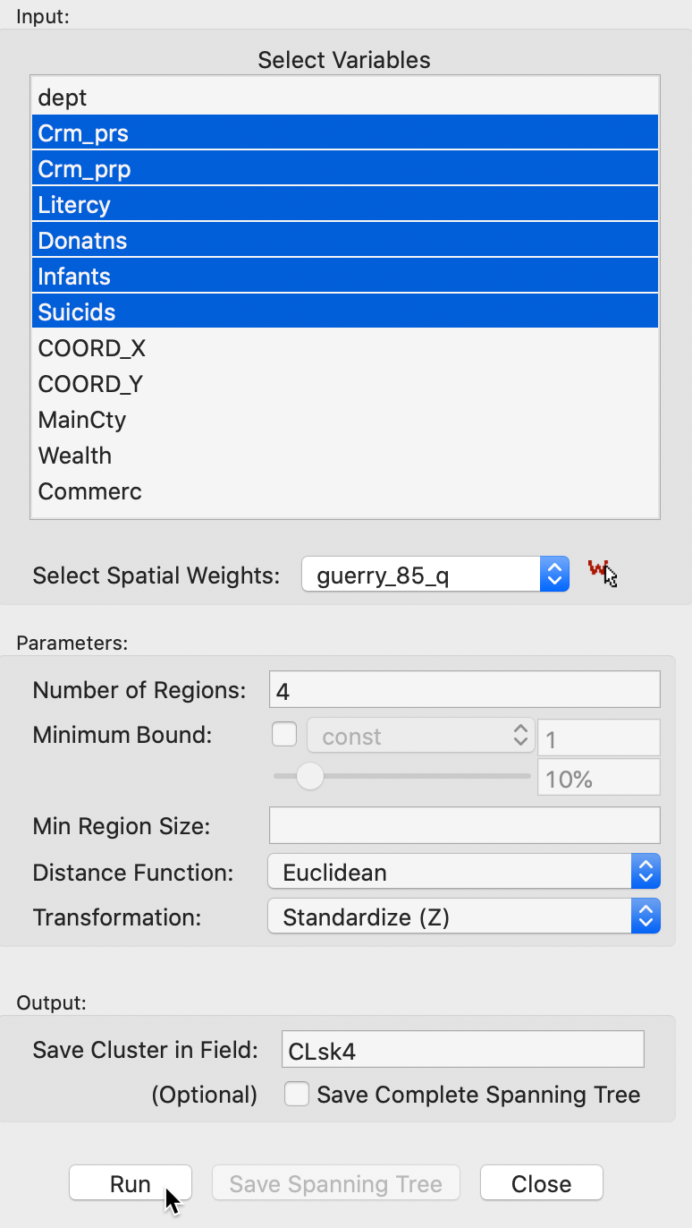
Figure 9: SKATER cluster settings

Clicking on Run brings up the SKATER cluster map as a separate window and lists the cluster characteristics in the Summary panel. We only give the map for now, as Figure 10, and consider the summary for k=6 below.

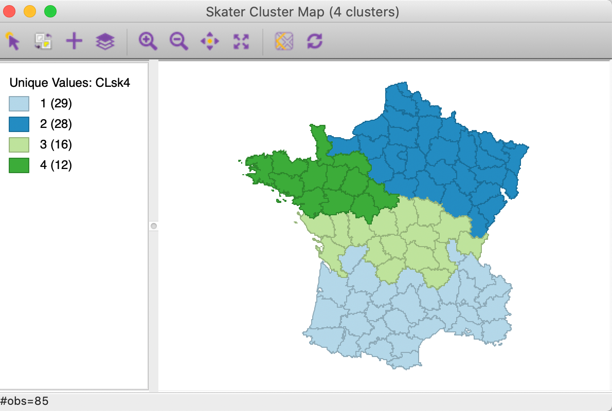
Figure 10: SKATER cluster map (k=4)

The spatial clusters generated by SKATER follow the minimum spanning tree closely and tend to reflect the hierarchical nature of the pruning. In this example, the country initially gets divided into three largely horizontal regions, of which the top one gets split into an eastern and a western part.

The hierarchical nature of the SKATER algorithm can be further illustrated by increasing the number of clusters to 6 for easier comparison with SCHC (all other options remain the same). The resulting cluster map in Figure 11 shows how the previous regions 3 and 4 each get split into an eastern and a western part.

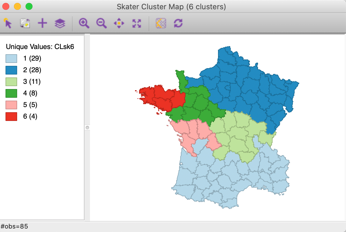
Figure 11: SKATER cluster map (k=6)

The summary in Figure 12 reveals a ratio of between sum or squares to total sum of squares of about 0.420. This is inferior to the result we obtained for SCHC for Ward’s method (about 0.462), but better than for the other linkage functions.

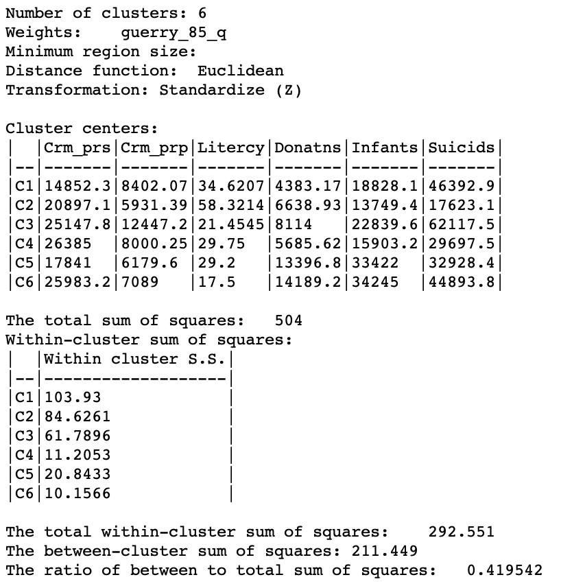
Figure 12: SKATER cluster summary (k=6)

Saving the minimum spanning tree

Near the bottom of the settings dialog is an option to save the minimum spanning tree. As shown in Figure 13, either the complete MST can be saved, with the corresponding box checked, or the MST that corresponds to the final result (box unchecked, the default).

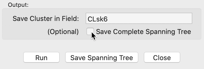
Figure 13: Minimum spanning tree options

The MST is saved as a gwt weights file and is loaded into the Weights Manager upon creation. This allows the graph to be displayed using the Connectivity > Show Graph option in the cluster map (or any map). In Figure 14, the complete MST is shown.⁵ We clearly see the edges that correspond with the transition between clusters.

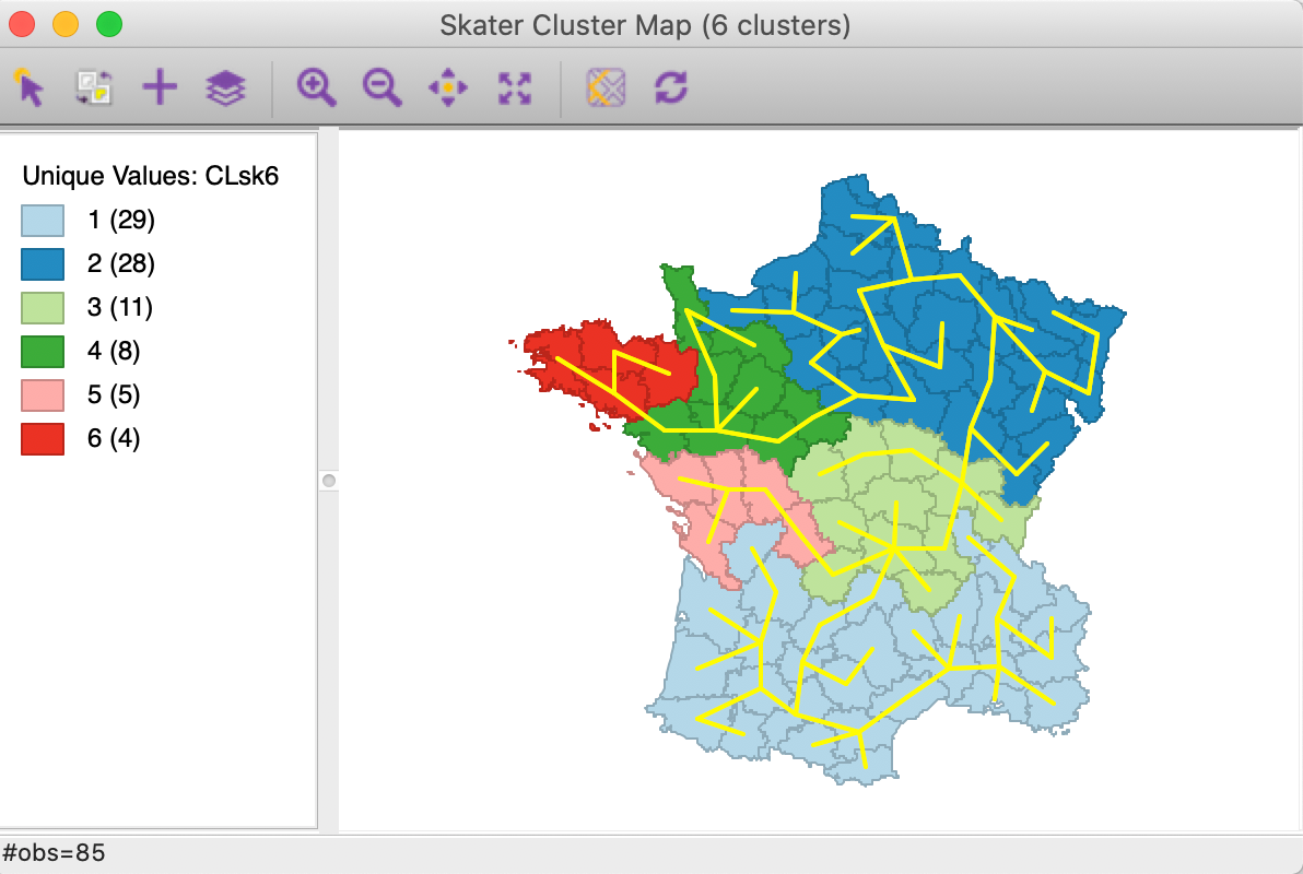
Figure 14: Complete minimum spanning tree

In Figure 15, these edges are removed and the MST corresponding with the final solution (for k=6) is displayed. This illustrates both the hierarchical nature of the algorithm as well as how the result follows from pruning the MST.

Figure 15: Minimum spanning tree for k=6

Since the MST is added to the Weights Manager as the last file, it becomes the default for future spatial analyses. This is typically not what one wants, so the active weight needs to be reset to a proper spatial weights definition before proceeding further.

Setting a minimum cluster size

In several applications of spatially constrained clustering, a minimum cluster size needs to be taken into account. For example, this is the case when the new regional groupings are intended to be used in a computation of rates. In those instances, the denominator should be sufficiently large to avoid extreme variance instability, which is accomplished by setting a minimum population size.

In GeoDa, there are two options to implement this additional constraint. One is through the Minimum Bound settings, as shown in Figure 16. The check box activates a drop down list of variables where a spatialy extensive variable can be selected for the minimum bound constraint, such as the population (or, in other examples, total number of households, housing units, etc.). In our example, we select the departmental population, Pop1831. The default is to take 10% of the total over all observations as the minimum bound. This can be adjusted by means of a slider bar (to set the percentage), or by typing in a different value in the minimum bound box. Here, we take the default.

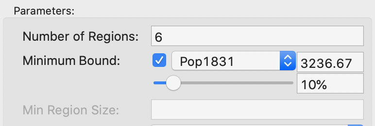
Figure 16: SKATER minimum bound settings

The resulting spatial alignment of clusters is quite different from the unconstrained solution, but again can be seen to be the result of a hierarchical subdivision of the three large horizontal subregions. As shown in the left panel of Figure 17, the northernmost region is divided into three, and the southernmost one into two subregions. Compared to the unconstrained solution, where the clusters consisted of 29, 28, 11, 8, 5, and 4 departments, the constrained regions have a much more even distribution of 21, 17, 16, and 12 (twice) and 7 elements.

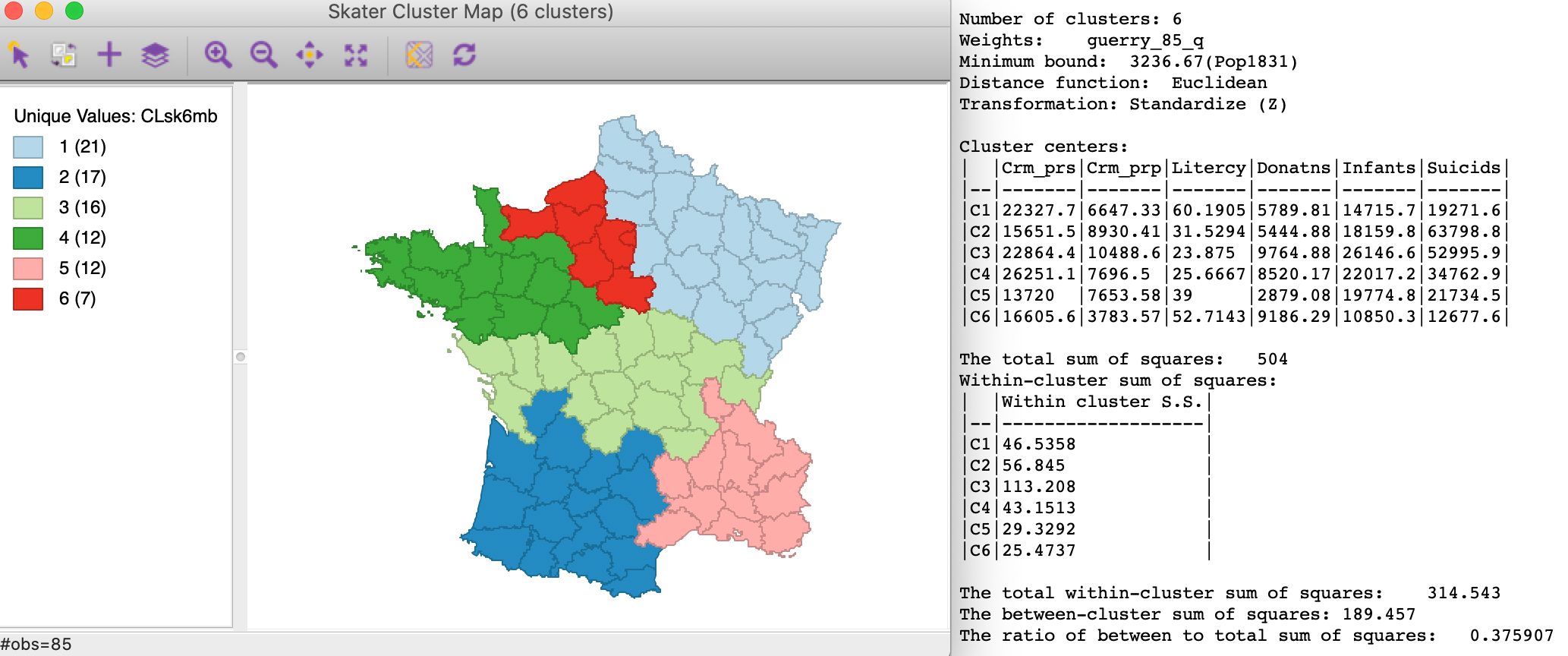
Figure 17: SKATER cluster map, min pop 10% (k=6)

The effect of the constraint is to lower the objective function from 0.420 to 0.376. The within-cluster sum of squares of the six regions is much more evenly distributed than in the unconstrained solution, due to the similar number of elements in each cluster.

The second way to constrain the regionalization process is to specify a minimum number of units that each cluster should contain. Again, this is a way to ensure that all clusters have somewhat similar size, although it is not based on a substantive variable, only on the number of elemental units. The constraint is set in the Min Region Size box of the parameters panel in Figure 16. In our example, we set the value to 12.

The result is slighlty different from that generated by the minimum population constraint. As shown in Figure 18, we now have the three smallest clusters with size 12 (as mandated by the constraint). The ratio of between to total sum of squares is slightly inferior at 0.374.

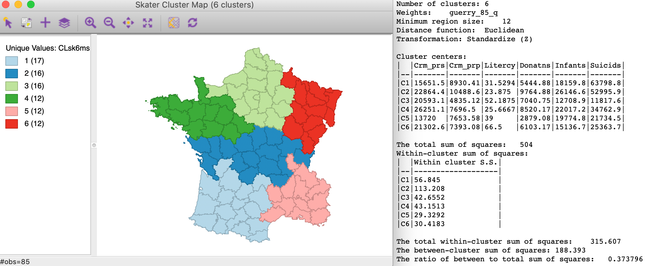
Figure 18: SKATER cluster map, min size 12 (k=6)

Note that the minimum region size setting will override the number of clusters when it is set too high. For example, setting the minimum cluster size to 14 will only yield clusters with k=5. Again, this is a consequence of the hierarchical nature of the minimum spanning tree pruning used in the skater algorithm. More specifically, a given sub-tree may not have sufficient nodes to allow for further subdivisions that meet the minimum size requirement. A similar problem occurs when the mininum population size is set too high.

REDCAP

Principle

Whereas SCHC involves an agglomerative hierarchical approach and SKATER takes a divisive perspective, the REDCAP collection of methods suggested by Guo (2008) combines the two ideas (see also Guo and Wang 2011). In this, a distinction is made between the linkage update function (originally, single, complete and average linkage), and between the treatment of contiguity.

As Guo (2008) points out, the MST that is at the basis of the SKATER algorithm only takes into account first order contiguity among pairs of observations. Unlike what we saw in SCHC, the contiguity relations are not updated to consider the newly formed clusters. As a result of this, observations that are part of a cluster that borders on a given spatial unit are not considered to be neighbors of that unit unless they are also first order contiguous. The distinction between a fixed contiguity relation and an updated spatial weights matrix is called FirstOrder and FullOrder. As a result, there are six possible methods, combining the three linkage functions with the two views of contiguity. In later work, Ward’s linkage was implemented as well.

We already saw earlier in the discussion of density-based clustering how the single-linkage dendrogram corresponds with a minimum spanning tree (MST). As a result, REDCAP’s FirstOrder-SingleLinkage and SKATER are identical. Since the FirstOrder methods are generally inferior to the FullOrder approaches, the latter are the main focus in GeoDa (for comparison to SKATER, FirstOrder-SingleLinkage is included as well, but the other FirstOrder methods are not).

A careful consideration of the various REDCAP algorithms reveals that they essentially consist of three steps. First, a dendrogram for contiguity constrained hierarchical clustering is constructed, using the given linkage function. This yields the exact same dendrogram as produced by SCHC. Next, this dendrogram is turned into a spanning tree, using standard graph manipulation principles. Finally, the optimal cuts in the spanning tree are obtained using the same logic (and computations) as in SKATER, up to the desired level of k.

Implementation

The collection of REDCAP algorithms is invoked as the third item in the hierarchical group on the Clusters toolbar icon (Figure 1), or from the main menu as Clusters > redcap.

Selecting this option brings up the REDCAP Settings dialog, shown in Figure 19. This interface has the same structure as for SKATER, except that multiple methods are available. The panel provides a way to select the variables, the number of clusters and different options to determine the clusters. As for the previous methods, we again have a Weights drop down list, where the contiguity weights must be specified. The REDCAP algorithms do not work without a spatial weights file.

The Distance Function and Transformation options operate in the same manner as before. At the bottom of the dialog, we specify the Field or variable name where the classification will be saved. The Minimum Bound and Min Region Size options work in the same way as for SKATER and will not be considered separately here.

We continue with the Guerry example data set and select the same six variables as before: Crm_prs, Crm_prp, Litercy, Donatns, Infants, and Suicids. The spatial weights are based on queen contiguity (guerry_85_q) and the the number of clusters is set to 6.

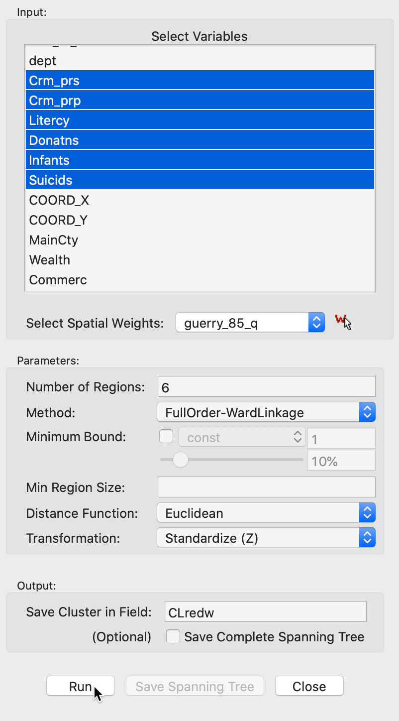
Figure 19: REDCAP cluster settings

Full-Order Ward’s linkage

We select the default method as FullOrder-WardLinkage, which implements Ward’s linkage with dynamically updated spatial weights. This yields the cluster map shown in the left-hand panel of Figure 20.

The results differ only marginally from the cluster map for SCHC using Ward’s linkage, shown in Figure 3. One department moves from the cluster containing eight units to the cluster in the south with 27 units, making the latter now the largest with 28 departments.

The cluster summary statistics, shown in the right-hand panel of Figure 20 are essentially the same as for the SCHC case, but slightly worse, with a between to total SS ratio of 0.460.

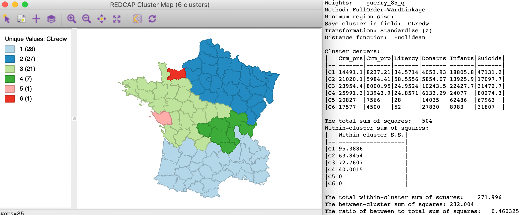
Figure 20: REDCAP Full Order, Ward’s linkage, k=6

As for SKATER, we can save the spanning tree associated with the linkage method, shown in Figure 21. There are some general similarities with the SKATER MST (Figure 14), but a close comparison reveals several important differences as well.

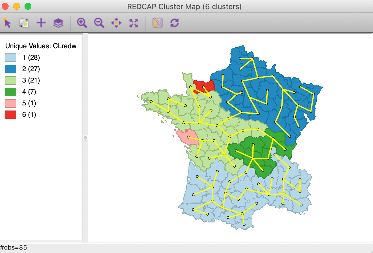
Figure 21: Spanning tree for REDCAP Full Order Ward’s linkage

The options for minimum size work in the same way as for SKATER and are not further considered.

For the sake of completeness, we show the results for the three other FullOrder linkage methods as well. GeoDa also includes FirstOrder-SingleLinkage, but the results are identical to those of SKATER and are not further reported here.

Full-Order Average linkage

The cluster map and summary characteristics of Full-Order Average linkage are shown in Figure 22. Compared to Ward’s results, the clusters are more balanced and there are no longer any singletons. The dominance of the large northern and southern clusters remains, but the departments in the middle of the country are arranged in different clusters. The ratio of between to total sum of squares is 0.429, somewhat worse than for Ward’s.

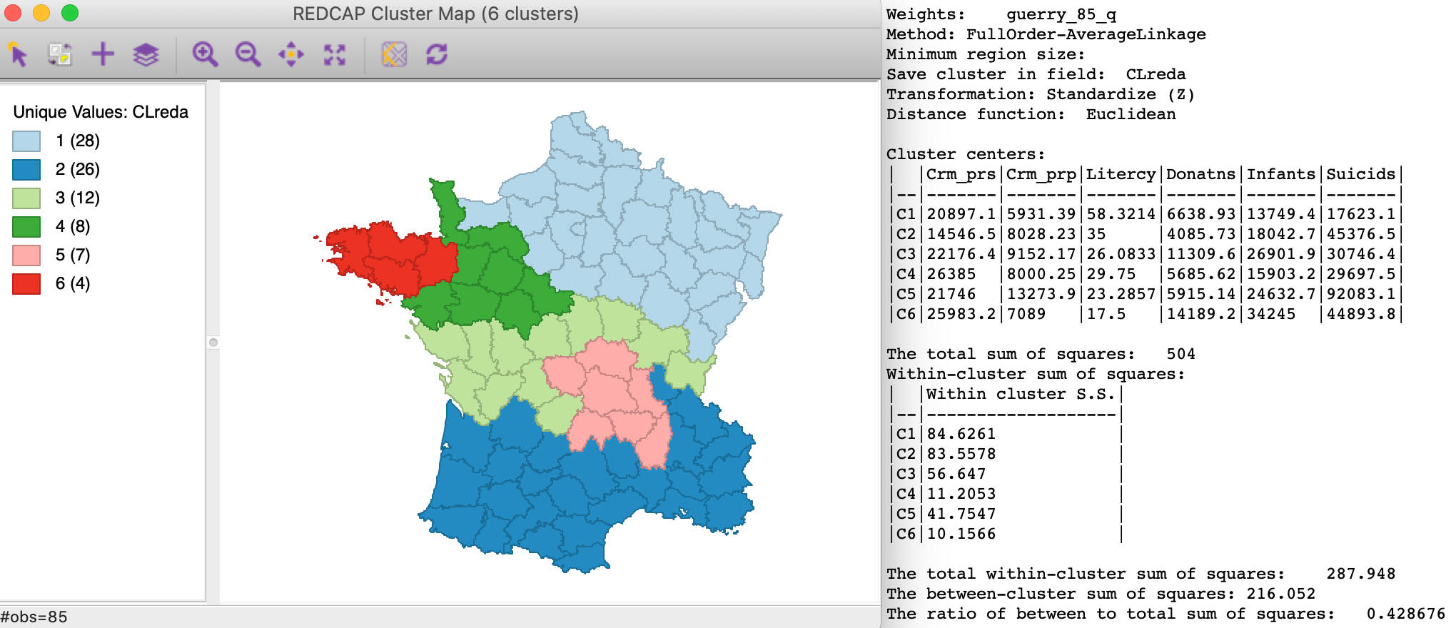
Figure 22: REDCAP Full Order, average linkage, k=6

Full-Order Complete linkage

The result for Full-Order Complete linkage is shown in Figure 23. We again have two singletons, one of which is in the same (northern) location as for Ward’s linkage, but the other one is not. As before, the main differences are for the departments in the middle of the country. The ratio of between to total sum of squares is slightly better than for average linkage, at 0.435.

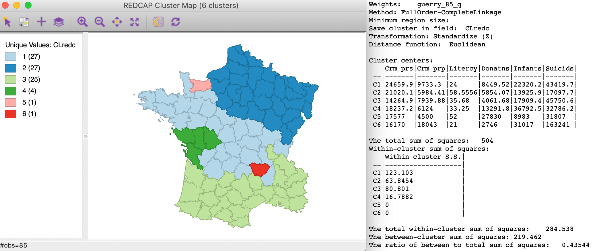
Figure 23: REDCAP Full Order, complete linkage, k=6

Full-Order Single linkage

Finally, the results for Full-Order Single linkage are the worst. As shown in Figure 24, the clusters share a singleton with Ward’s linkage and another cluster with average linkage, but otherwise the spatial pattern is quite distinct from the previous cases. The ratio of between to total sum of squares is the worst of the four options, at 0.388.

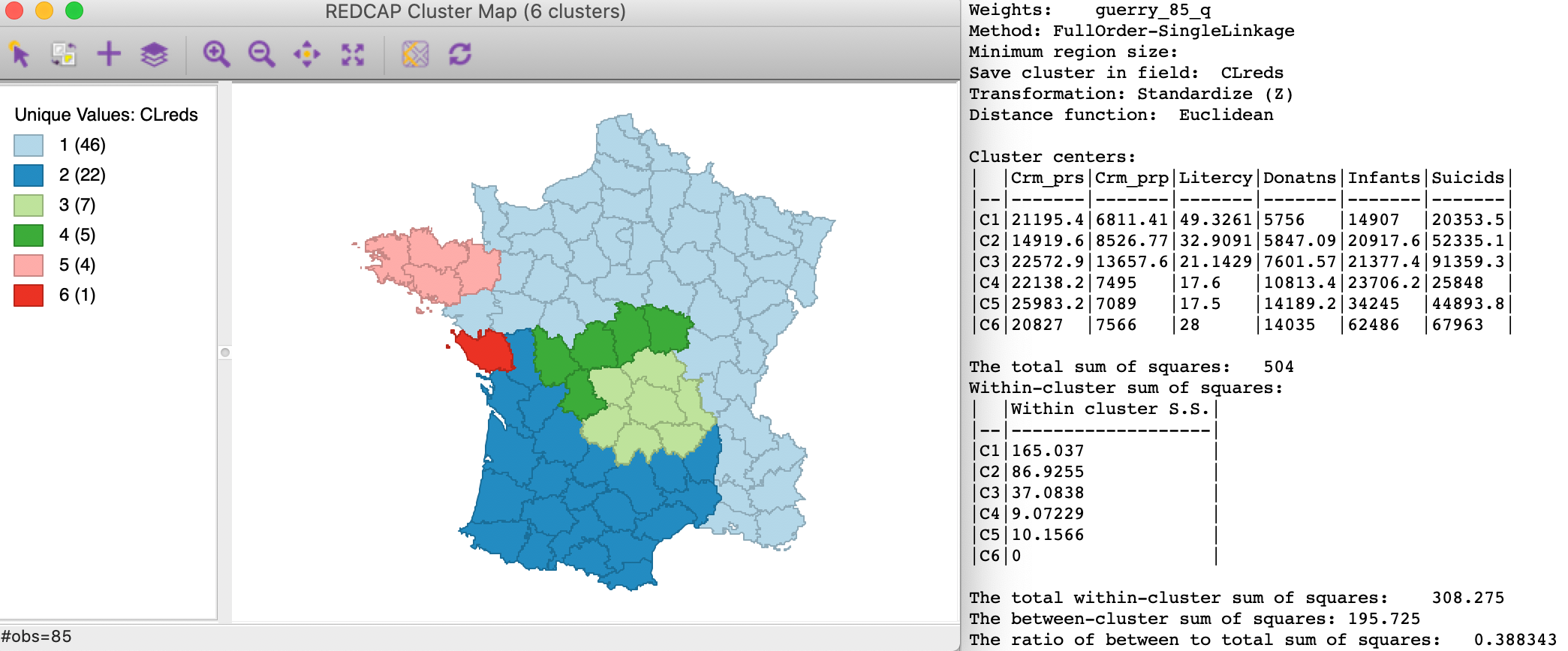
Figure 24: REDCAP Full Order, single linkage, k=6

Assessment

Clearly, different assumptions and different algorithms yield greatly varying results. This may be discomforting, but it is important to keep in mind that each of these approaches have a slightly different way to handle the tension between attribute and locational similarity.

In the end, the results can be evaluated on a number of different criteria. GeoDa reports the ratio of the between sum of squares to the total sum of squares, but that is only one of a number of possible metrics, such as compactness, balance, etc. Also, the commonalities and differences between the various approaches highlight where the tradeoffs are particularly critical.

Finally, it should be kept in mind that the solutions offered by the different algorithms have no guarantee to yield global optima. Therefore, it is important to consider more than one method, in order to gain insight into the sensitivity of the results to the approach chosen.

Appendix

Arizona counties sample data set

We will use a small enough data set to illustrate the various spatially constrained algorithms. As it turns out, the state of Arizona has only 14 counties, which is perfect for our purposes. We create this data set by starting with the natregimes data set and selecting the counties with STFIPS equal to 4, which are the counties in Arizona. If we then use Save Selected As we obtain the data set shown in Figure 25. We created a new variable AZID which gives an id to the counties in alphabetical order. This identifier is shown in Figure 25.

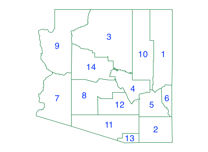
Figure 25: Arizona counties

To keep things simple, we will only use a single variable, the unemployment rate in 1990, UE90. We standardize this variable (using the Calculator) as SUE and show the associated values in Figure 26.

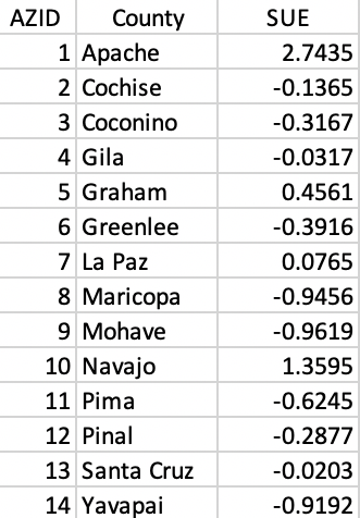
Figure 26: County identifiers and standardized variable

The final piece to complete our analysis is a spatial weight matrix. In Figure 27 we show the contents of the queen contiguity gal file.

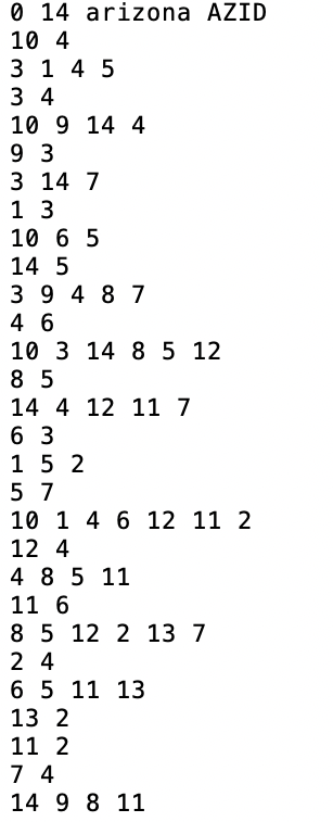
Figure 27: AZ county queen contiguity information

SCHC Complete Linkage worked example

We illustrate the spatially constrained hierarchical clustering using complete linkage. Even though this is not an ideal linkage selection, it is easy to implement and helps to illustrate the logic of the SCHC.

The point of departure is the matrix of Euclidean distance in attribute space. In our example, there is only one variable, so the distance is equivalent to the absolute difference between the values at two locations. In Figure 28, the full distance matrix is shown. Distinct from the example in the unconstrained case, we limit our attention to those pairs of observations that are spatially contiguous, shown highlighted in red in the matrix.

The first step is to identify the pair of observations that are closest in attribute space and contiguous (red in the table). Inspection of the distance matrix in Figure 28 finds the pair 8-14 as the least different, with a distance value of 0.03.

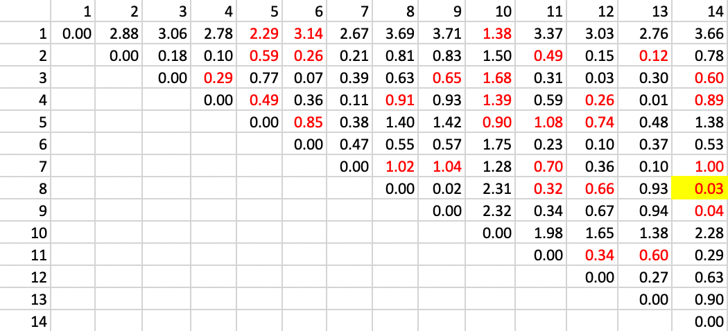
Figure 28: SCHC complete linkage step 1

The next step is to combine observations 8 and 14 and recompute the distance from other observations as the largest from either 8 or 14. The updated matrix is shown in Figure 29. In addition, the contiguity matrix must be updated with neigbors to the cluster 8-14 as those who were either neighbors to 8 or 14, or to both. The updated neighbor relation is shown as the red values in the matrix. The smallest value is between 9 and 8-14, which yields a new cluster of 8-9-14.

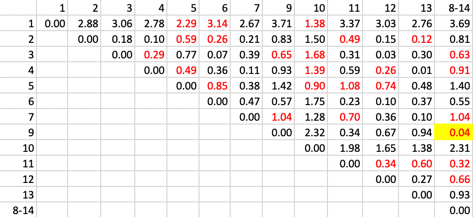
Figure 29: SCHC complete linkage step 2

The remaining steps proceed in the same manner. The contiguity relations are updated and the largest distance between the two elements of the cluster is entered as the new distance in the matrix. In step 3, shown in Figure 30, we identify the pair with the smallest value of 0.12, between 2 and 13, which is our new cluster.

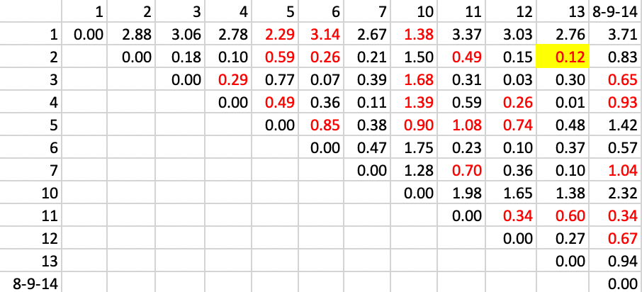
Figure 30: SCHC complete linkage step 3

With the updated contiguities, step 4 identifies the pair 4-12 as the new cluster, with a distance of 0.26, as in Figure 31.

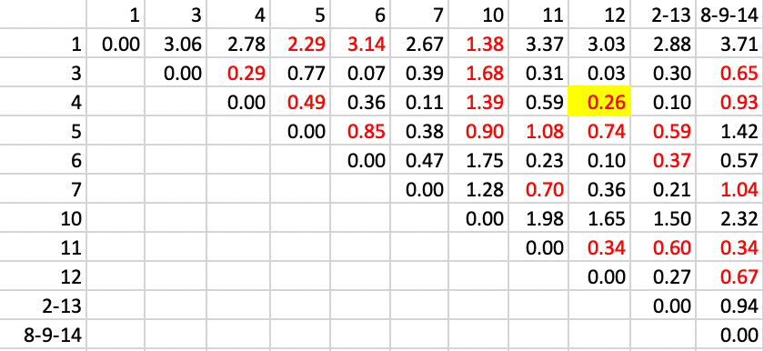
Figure 31: SCHC complete linkage step 4

We continue in the same way with step 5, identifying a new cluster of 3-4-12 with a distance of 0.29.

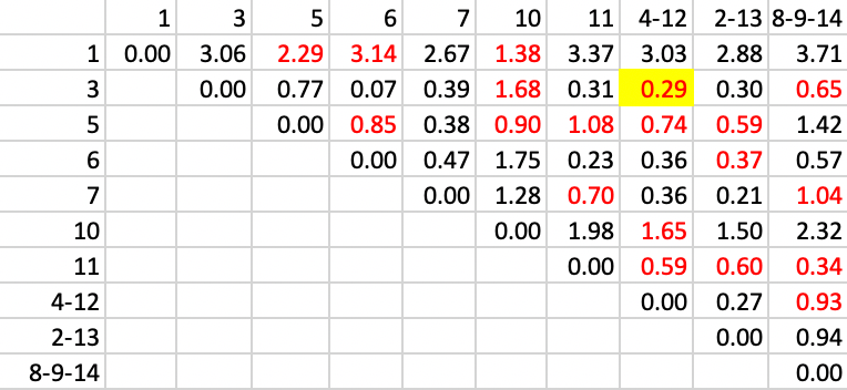
Figure 32: SCHC complete linkage step 5

In step 6, we add 11 to the existing cluster of 8-9-14, with a distance of 0.34, as shown in Figure 33.

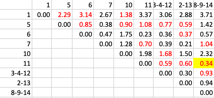
Figure 33: SCHC complete linkage step 6

Next, we add 6 to 2-13, with a distance of 0.37, as in Figure 25.

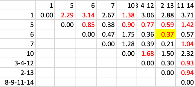
Figure 34: SCHC complete linkage step 7

Now, 5 joins 3-4-12, with a distance of 0.77, in Figure 35.

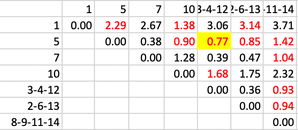
Figure 35: SCHC complete linkage step 8

The final few steps continue to reduce the number of clusters. In this stage, the two clusters 3-4-5-12 and 2-6-13 are joined, with a distance of 0.85, as in Figure 36.

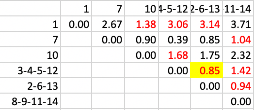
Figure 36: SCHC complete linkage step 9

Next, 7 is added to 8-9-11-14, with a distance of 1.04, in Figure 37.

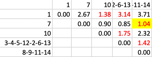
Figure 37: SCHC complete linkage step 10

At this point, 1 and 10 are joined, with a distance of 1.38, shown in Figure 38.

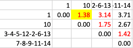
Figure 38: SCHC complete linkage step 11

The next to final step, resulting in two clusters, merges 3-4-5-12-2-6-13 with 7-8-9-11-14, with a distance of 1.42, as in Figure 39.

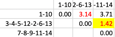
Figure 39: SCHC complete linkage step 12

One interesting aspect of these steps is that at each stage, the distance involved is larger. As mentioned above, the complete linkage approach avoids the inversion problem, so that we indeed see a uniform increase in the distances involved.

We can also visualize the process by the dendrogram generate by GeoDa for this example, shown in Figure 40. We see from the distance associated with each pair how the first merger is between 8 and 14, followed by adding 9, etc. The steps in the dendrogram identically follow the steps illustrated above.

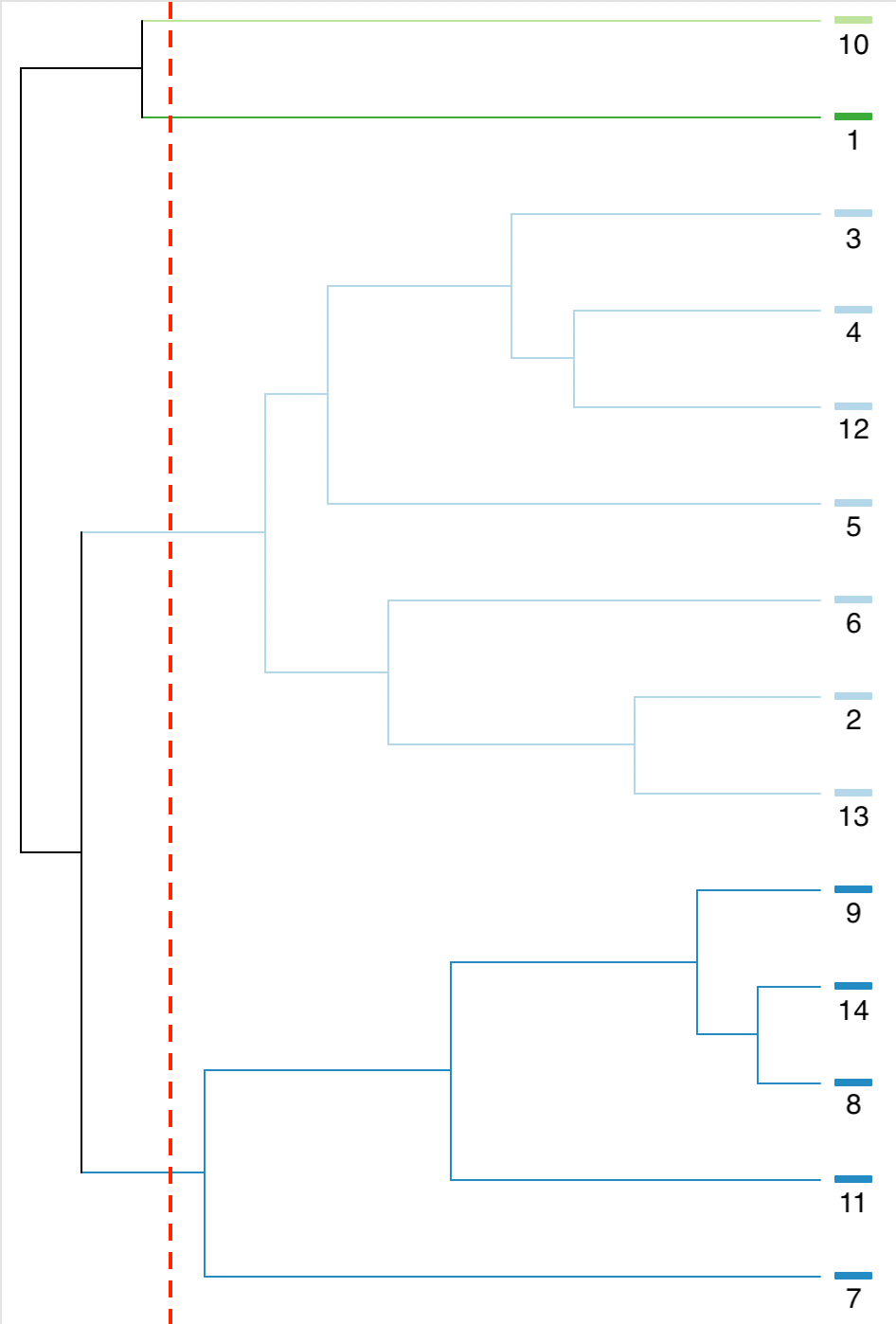
Figure 40: SCHC complete linkage dendrogram, k=4

Finally, we show the spatial layout of the clusters for k=4 in Figure 41. Clearly, the contiguity constraint has been satisfied.

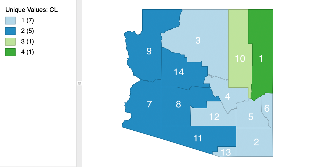
Figure 41: SCHC complete linkage cluster map, k=4

SKATER worked example

We illustrate the SKATER algorithm with the same Arizona county example, with k (the number of clusters) set to 4. In Figure 42, we list the observations and their squares, which form the basis for the computation of the relevant sums of squared deviations (SSD) for each subset.

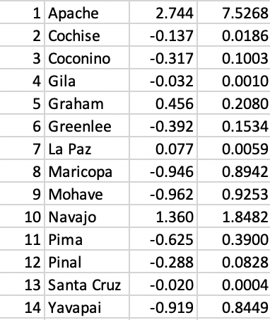
Figure 42: AZ county variables

The first step in the process is to reduce the information for contiguous pairs in the distance matrix of Figure 28 (shown in red) to a minimum spanning tree (MST). The result is shown in Figure 43, against the backdrop of the Arizona county map.

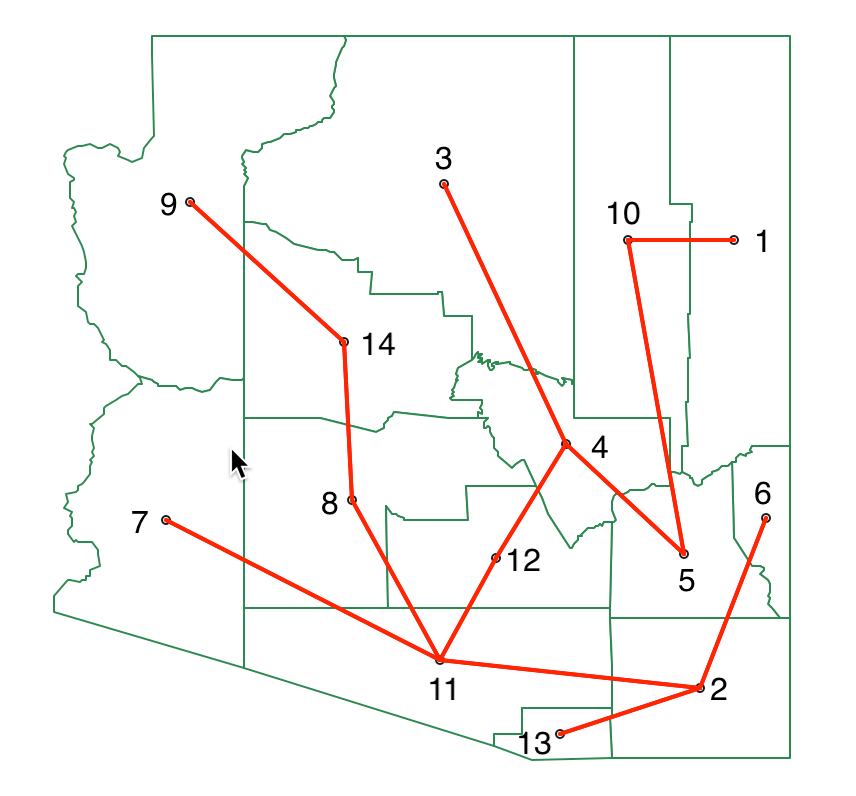
Figure 43: SKATER minimum spanning tree

We now have to evaluate every possible cut in the MST in terms of its contribution to reducing the overall sum of squared deviations (SSD). We know the data in third column of Figure 42 is standardized, so the mean is zero by construction. As a result, the total sum of squared deviations is the sum of squares, i.e., the sum of the values listed in the fourth column. This sum is 13.000 (rounded).⁶

The vertices for each possible cut are shown as the first two columns in Figure 44. For each subtree, we need to compute the corresponding SSD. The next step then implements the optimal cut such that the total SSD decreases the most, i.e., max[\(\mbox{SSD}_T - (\mbox{SSD}_a + \mbox{SSD}_b)\)], where \(\mbox{SSD}_T\) is the SSD for the corresponding tree, and \(\mbox{SSD}_a\) and \(\mbox{SSD}_b\) are the totals for the subtrees corresponding to the cut.

In order to accomplish this, we first compute the mean of the values associated with the vertices of each subtree, and then calculate the SSD for each subtree k as \(\sum_i x_i^2 - n_k \bar{x}_k^2\), with \(\bar{x}_k\) as the mean for the average value for the subtree and \(n_k\) as the number of elements in the subtree.

In the interest of space, we do not show all the calculations, but give a few examples. For the cut 1-10, the vertex 1 becomes a singleton, so its SSD is 0 (\(SSD_a\) in the fourth column and first row in Figure 44). For vertex 10, the subtree consists of all 13 elements other than 1, with a mean of -0.211 and an SSD of 4.894 ( \(SSD_b\) in the fifth column and first row in Figure 44). Consequently, the contribution to reducing the overall SSD amounts to 13.000 - (0 + 4.894) = 8.106.

In a similar fashion, we compute the SSD for each possible subtree and enter the values in Figure 44. The largest decrease in overall SSD is achieved by the cut between 5 and 10, which yields a reduction of 9.820.

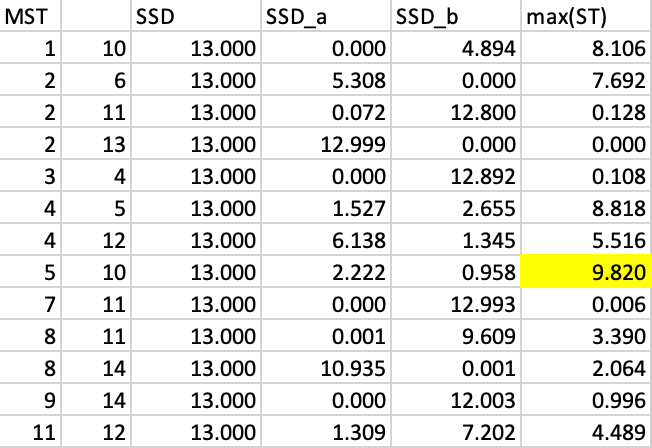
Figure 44: SKATER step 1

The new MST after cutting the link between 5 and 10 is shown in Figure 45, yielding two initial clusters.

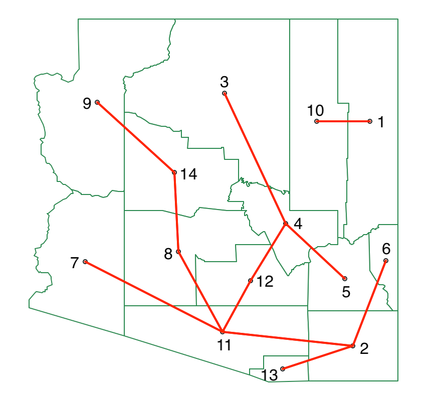
Figure 45: SKATER minimum spanning tree - first split

We now repeat the process, looking for the greatest decrease in overall SSD. We separate the data into two subtrees, one for 1-10 and the other for the remaining vertices. In each, we recalculate the SSD for the subtree, which yields 0.958 for 1-10 and 2.222 for the other cluster. For each possible cut, we compute the SSD for the corresponding subtrees, with the results shown in Figure 46. At this point, the greatest contribution towards reducing the overall SSD is offered by a cut between 8 and 11, with a contribution of 1.441.

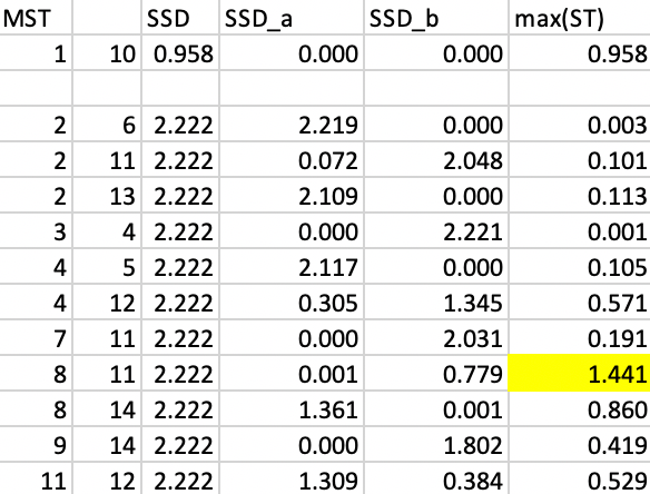
Figure 46: SKATER step 2

The corresponding MST for the three clusters is shown in Figure 47. We now have one cluster of two units, one with three, and one with nine.

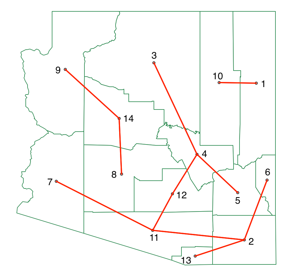
Figure 47: SKATER minimum spanning tree - second split

At this point, we only need to make one more cut (k=4). When we compute the SSD for each subtree, we find a total of 0.0009 for 8-9-14, and a value of 0.779 for the remainder, both well below the contribution to decreasing the SSD of 0.958 obtained by 1-10 (since the split yields two single observations, the decrease in SSD equals the total SSD for the subtree). Consequently, we do not need to carry out the detailed calculations for each other subtree, since the final cut is between 1 and 10, yielding two singletons. As a result, we have four clusters, with the final MST shown in Figure 48.

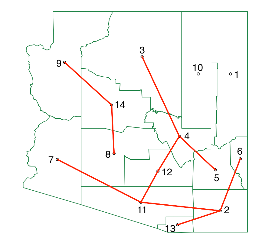
Figure 48: SKATER minimum spanning tree - third split

The matching cluster map created by GeoDa for SKATER with k=4 is shown in Figure 49. The four regions match the subtrees in the MST, with 1 and 10 being singletons.

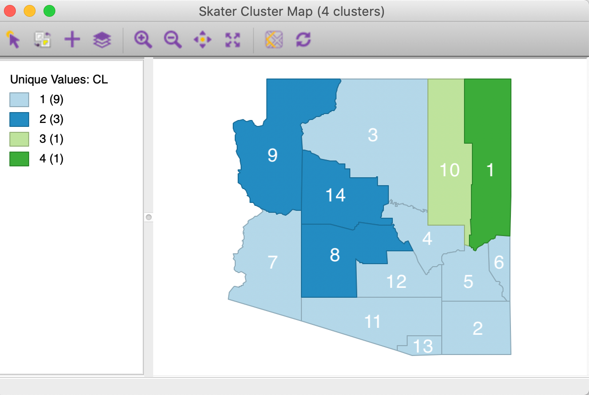
Figure 49: SKATER cluster map, k=4

REDCAP worked example

We now use the Arizona counties example to illustrate the logic of the REDCAP FullOrder-CompleteLinkage option. As it turns out, we can reuse the results from SCHC and the logic from SKATER.

The first stage in the REDCAP algorithm is to construct a spanning tree that corresponds to a spatially constrained complete linkage hierarchical clustering dendrogram.

In our illustration, we implement FullOrder, i.e., the contiguity relations between clusters is dynamically updated. Consequently, the steps to follow are the same as for complete linkage SCHC, yielding the dendrogram in Figure 40.

To create a spanning tree representation of this dendrogram, we connect the observations following the merger of entities in the dendrogram. In our example, this means we first connect 8 and 14. In the second step, we connect 9 to the cluster 8-14, but since 9 is only contiguous to 14, we make the edge 9-14. The full sequence of edges is given in the list below. Whenever we connect a new entity to a cluster, we either connect it to the only contiguous unit, or to the contiguous one that is closest (using the distance measures in Figure 28 ):

• Step 1: 8-14
• Step 2: 9-14
• Step 3: 2-13
• Step 4: 4-12
• Step 5: 3-4
• Step 6: 11-8
• Step 7: 6-2
• Step 8: 5-4
• Step 9: 2-5
• Step 10: 7-11
• Step 11: 1-10
• Step 12: 11-12
• Step 13: 10-5

The resulting spanning tree is shown in Figure 50, with the sequence of steps marked in blue. The tree is largely the same as the MST in Figure 43, except that the link between 11 and 2 is replaced by a link between 5 and 2.

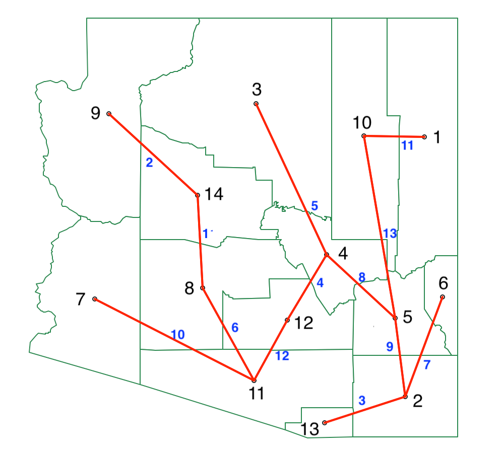
Figure 50: REDCAP FullOrder-CompleteLinkage spanning tree

At this point, we search for an optimal cut using the same approach as for SKATER. Given the similarity of the two trees, we will be able to reuse a lot of the previous results. Only those subtrees affected by the new link 5-2 replacing the link 11-2 need to be considered again. Specifically, in the first step, these are the edges 5-2, 5-4, 4-12 and 11-12. The other results can be borrowed from the first step in SKATER, shown in Figure 44. The new results are given in Figure 51. As in the SKATER case, the first cut is between 5 and 10.

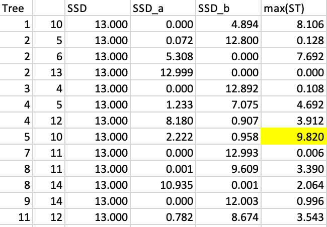
Figure 51: REDCAP step 1

We proceed in the same manner for the second step, where again we can borrow several results directly from the SKATER case. Figure 52 lists the updated values. Here again, the optimal cut is between 8 and 11.

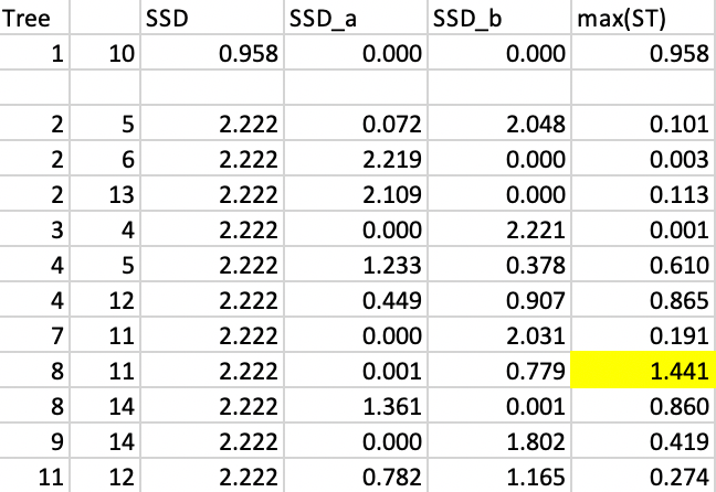
Figure 52: REDCAP step 2

The final step is the same as for SKATER, yielding the same layout as in Figure 49 for our four clusters.

References

Assunção, Renato M., M. C. Neves, G. Câmara, and C. Da Costa Freitas. 2006. “Efficient Regionalization Techniques for Socio-Economic Geographical Units Using Minimum Spanning Trees.” International Journal of Geographical Information Science 20 (7): 797–811.

Duque, Juan Carlos, Raúl Ramos, and Jordi Suriñach. 2007. “Supervised Regionalization Methods: A Survey.” International Regional Science Review 30: 195–220.

Duque, Juan C., Richard L. Church, and Richard S. Middleton. 2011. “The p-Regions Problem.” Geographical Analysis 43: 104–26.

Gordon, A. D. 1996. “A Survey of Constrained Classification.” Computational Statistics and Data Analysis 21: 17–29.

Guo, Diansheng. 2008. “Regionalization with Dynamically Constrained Agglomerative Clustering and Partitioning (REDCAP).” International Journal of Geographical Information Science 22 (7): 801–23.

———. 2009. “Greedy Optimization for Contiguity-Constrained Hierarchical Clustering.” In 2013 IEEE 13th International Conference on Data Mining Workshops, 591–96. Los Alamitos, CA, USA: IEEE Computer Society. https://doi.org/10.1109/ICDMW.2009.75.

Guo, Diansheng, and Hu Wang. 2011. “Automatic Region Building for Spatial Analysis.” Transactions in GIS 15: 29–45.

Lankford, Philip M. 1969. “Regionalization: Theory and Alternative Algorithms.” Geographical Analysis 1: 196–212.

Murray, Alan T., and Tony H. Grubesic. 2002. “Identifying Non-Hierarchical Spatial Clusters.” International Journal of Industrial Engineering 9: 86–95.

Murtagh, Fionn. 1985. “A Survey of Algorithms for Contiguity-Constrained Clustering and Related Problems.” The Computer Journal 28: 82–88.

Recchia, Anthony. 2010. “Contiguity-Constrained Hierarchical Agglomerative Clustering Using SAS.” Journal of Statistical Software 22 (2).

---

1. University of Chicago, Center for Spatial Data Science – anselin@uchicago.edu↩︎

2. This skater algorithm is not to be confused with tools to interpret the results of deep learning https://github.com/oracle/Skater.↩︎

3. This can readily be computed as \(\sum_i x_i^2 - n_T \bar{x}_T^2\), where \(\bar{x}_T\) is the average for the subtree, and \(n_T\) is the number of nodes in the subtree.↩︎

4. While this exhaustive evaluation of all potential cuts is inherently slow, it can be speeded up by exploiting certain heuristics, as described in Assunção et al. (2006). In GeoDa, we use full enumeration, but implement parallelization to obtain better performance.↩︎

5. To obtain this graph, use Change Edge Thickness > Strong and set the color to yellow.↩︎

6. Since the variable is standardized, the estimated variance \(\hat{\sigma}^2 = \sum_i x_i^2 / (n - 1) = 1\). Therefore, \(\sum_i x_i^2 = n - 1\), or 13 in our example.↩︎

GeoDa is maintained by lixun910. This page was generated by GitHub Pages using the Cayman theme by Jason Long.