Spatial Data Wrangling (1) – Basic Operations

Introduction

In this and the following two chapters, we tackle the topic of data wrangling, i.e., the process of getting data from its raw input into a form that is amenable for analysis. This is often considered to be the most time consuming part of a data science project, taking as much as 80% of the effort (Dasu and Johnson 2003). Even though the focus in these notes is on analysis and not on data manipulation per se, we provide a quick overview of the functionality contained in GeoDa to assist with these operations. Increasingly, data wrangling has evolved into a field of its own, with a growing number of operations turning into automatic procedures embedded into software (Rattenbury et al. 2017). A detailed discussion of this is beyond our scope.

In the current chapter, we focus on essential input operations and data manipulations included in the Table functionality of GeoDa, including data queries. The second chapter in the series covers basic GIS operations. In the third chapter, we work through an extensive illustration using an example of information from an open data portal.

Objectives

• Load a spatial layer from a range of formats

• Convert between spatial formats

• Create a point layer from coordinates in a table

• Create a grid layer

• Become familiar with the table options

• Use the Calculator Tool to create new variables

• Variable standardization

• Merging tables

• Use the Selection Tool to select observations in a table

• Use a selection shape to select observations in a map

GeoDa functions covered

• File > Open
• File > Save As
• Tools > Shape > Points from Table
• Tools > Shape > Create Grid
• Table > Edit Variable Properties
• Table > Add Variable
• Table > Delete Variable(s)
• Table > Rename Variable
• Table > Encode
• Table > Setup Number Formatting
• Table > Move Selected to Top
• Table > Calculator
• Table > Selection Tool
• File > Save Selected As
• Map > Unique Values Map
• Map > Selection Shape
• Map > Save Selection

Preliminaries

We will illustrate the basic data input operations by means of a series of example data sets, all contained in the GeoDa Center data set collection.

Specifically, we will use files from the following data sets:

• Chicago commpop: population data for 77 Chicago Community Areas in 2000 and 2010

• Groceries: the location of 148 supermarkets in Chicago in 2015

• Natregimes: homicide and socio-economic data for 3085 U.S. counties in 1960-1990

• SanFran Crime: San Francisco crime incidents in 2012 (point data)

Make sure to have these data sets downloaded, unzipped and available in a working directory for analysis.

Spatial Data

Spatial data are characterized by the combination of two important aspects. First, there is information on traditional variables just as in any other statistical analysis. In the spatial analysis world, this is referred to as attribute information. Typically, this is contained in a flat (rectangular) table with observations as rows and variables as columns.

The second aspect of spatial data is distinct, and is referred to as locational information. This consists of the precise definition of spatial objects, classified as points, lines or areas. In essence, the formal characterization of any spatial object boils down to the description of x,y coordinates of points in space, as well as of a mechanism that spells out how these points are combined into spatial entities.

For a single point, this simply consists of its coordinates. For areal units, such as census tracts, counties, or states, the boundary is defined as a series of line segments, each characterized by the coordinates of their starting and ending points. In other words, what may seem like a continuous boundary, is turned into discrete segments.

Traditional data tables have no problem including x and y coordinates as columns, but as such cannot deal with the boundary definition of irregular spatial units. Since the number of line segments defining an areal boundary can easily vary from observation to observation, there is no efficient way to include this in a fixed number of columns of a flat table. Consequently, a specialized data structure is required, typically contained in a geographic information system or GIS.

Several specialized formats have been developed to efficiently combine both the attribute information and the locational information. Such spatial data can be contained in files with a special structure, or in spatially enabled relational data base systems.

In this section, we first consider common GIS file formats as input to GeoDa. We next illustrate simple tabular input of non-spatial files. We close with a brief overview of connections to other input formats.

GIS files

Historically, a wide range of different formats have been developed for GIS data, both proprietary as well as open source. In addition, there has been considerable effort at standardization, led by the Open Geospatial Consortium (OGC). GeoDa leverages the open source GDAL library to support many of the most popular formats in use today.

While it is impossible to cover all of these specifications in detail, we will illustrate the use of the proprietary shape file format of ESRI, the open source GeoJSON format, and the Geography Markup Language of the OGC as a standard XML grammar for defining geographical features.

GeoDa can load both polygon and point GIS data, but in the current implementation, line files (e.g., representing road networks) are not supported.

Spatial file formats

Arguably, the most familiar proprietary spatial data format is the shape file format, developed by ESRI. The terminology is a bit confusing, since there is no such thing as one shape file, but there is instead a collection of three (or four) files. One file has the extension .shp, one .shx, one .dbf, and one .prj (with the projection information). The first three are required, the fourth one is optional, but highly recommended. The files should all be in the same directory and have the same file name.

In the open source world, an increasingly common format is GeoJSON, the geographic augmentation of the JSON standard, which stands from JavaScript Object Notation. This format is contained in a text file and due to its highly structured nature is easy for machines to read.

Finally, the GML standard, or geographic markup language, is a XML implementation that prescribes the formal description of geographic features.

A detailed discussion of the individual formats is beyond our scope, but they are well-documented. For our purposes, there is no need to know the underlying formats, since the interaction with the data structures is handled by GeoDa under the hood.

The main file manipulations are invoked from the File item in the menu, or by one of the left-most icons on the toolbar, shown in Figure 1.

Figure 1: Toolbar icons for file manipulation

Polygon layers

Most of the analyses covered in these chapters will pertain to areal units, or polygon layers. We load these by invoking File > Open File from the menu, or by clicking on the left-most Open icon on the toolbar in Figure 1.

This brings up the Connect to Data Source dialog, shown in Figure 2. The left panel has File as the active input format. Other formats are Database and Web, which we briefly cover below. The right panel shows a series of Sample Data data are included with GeoDa. After some files have been loaded, the Recent panel lists their file names. Files listed in either panel can be loaded by simply clicking on their icon.

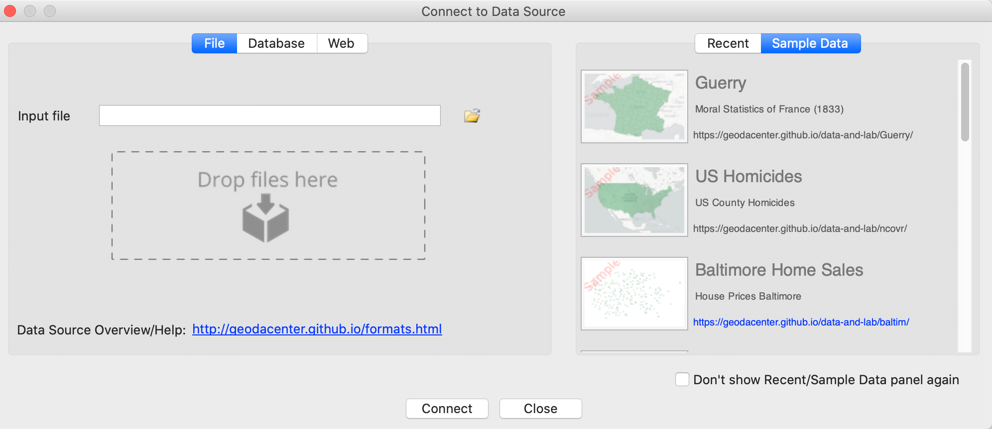
Figure 2: Connect to Data Source dialog

When clicking on the small folder icon to the right of the Input file box, a list of supported file formats appears, as in Figure 3. In this first example, we select the top item in the list, ESRI Shapefile (*.shp).

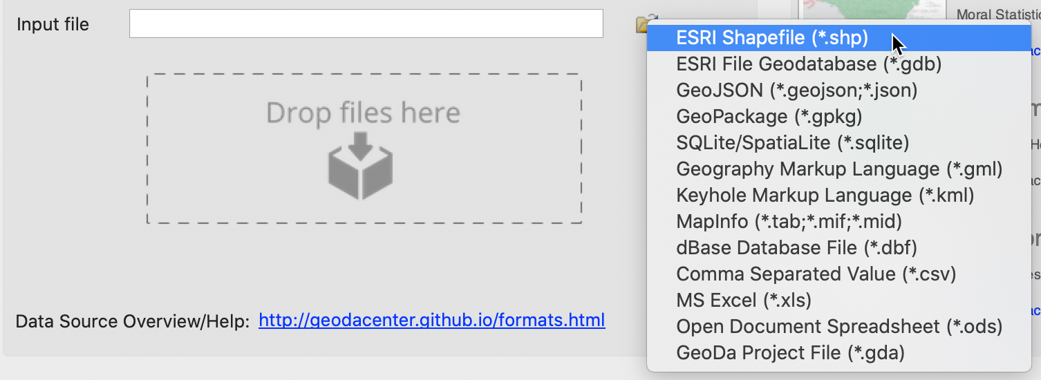
Figure 3: Supported spatial file formats

Next comes the familiar directory navigation dialog, specific to each operating system. After moving to the proper folder and selecting commpop.shp, a map window opens up with the spatial layer represented as a themeless choropleth map with 77 observations (listed in the top left). In our example, this is as in Figure 4.

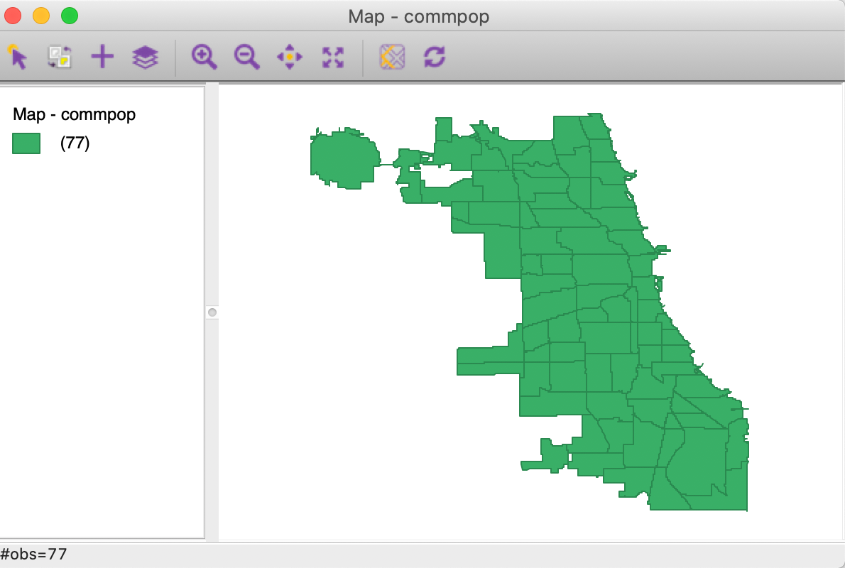
Figure 4: Themeless polygon map

We clear the current layer by clicking on the Close toolbar icon, the second item on the left. This removes the base map and the icon becomes inactive.

A more efficient way to open files is to select and drag the file onto the Drop files here box in the dialog.

Before we proceed with this, consider the contents of the file chicago_comm.geojson. In contrast to the shape file format, which is binary, a GeoJSON file is simple text and can easily be read by humans. As shown in Figure 5, we see how the locational information is combined with the attributes. After some header information follows a list of features. Each of these contains properties, of which the first set consists of the different variable names with the associated values, just as would be the case in any standard data table. However, the final item refers to the geometry. It includes the type, here a MultiPolygon, followed by a list of x-y coordinates. In this fashion, the spatial information is integrated with the attribute information.

Figure 5: Example GeoJSON file contents

To view the corresponding map, we select the chicago_comm.geojson file and drag it onto the Drop files here box. This brings up the same base map as in Figure 4.

File format conversion

The file we just loaded was in GeoJSON format. Let’s say we want to convert this into GML. This is accomplished in GeoDa by means of Save As and selecting Geographic Markup Language (*.gml) from the drop down list shown in Figure 3.

For example, if we save the file as commpop.gml, it is converted to the GML XML format, as illustrated in Figure 6. We notice the characteristic < > and </ > delimiters of the markup elements. In our file snippet, the top lines pertain to the geography of the first polygon, ended by </ogr:geometryProperty>. Next follow the actual observations with variable names and associated values, finally closed off with </gml:featureMember>. After this, a new observation is given, delineated by the <gml:featureMember> tag, followed by the geographic characteristics. Again, this illustrates how spatial information is combined with attribute information in an efficient file format.

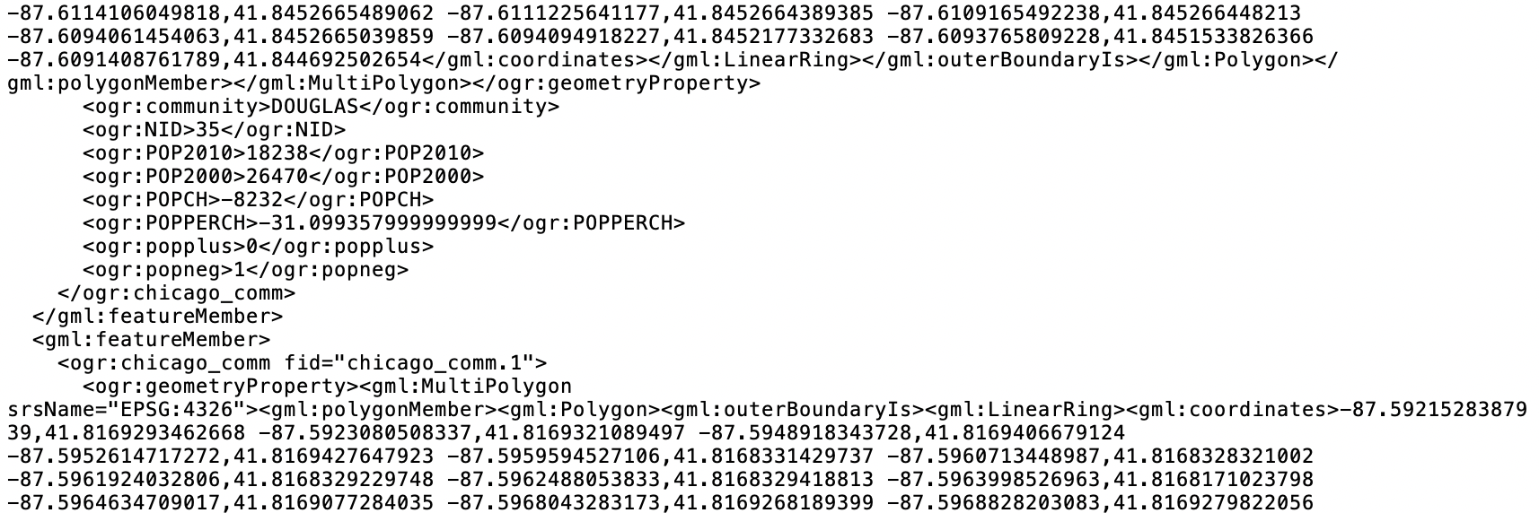
Figure 6: Example GML file contents

The Save As feature in GeoDa turns it into an effective GIS format converter.

Point layers

Point layer GIS files are loaded in the same fashion. For example, we can drag the file chicago_sup.shp from the Grocery sample data folder onto the Drop files here box. This generates a point map of 148 supermarket locations, as in Figure 7.

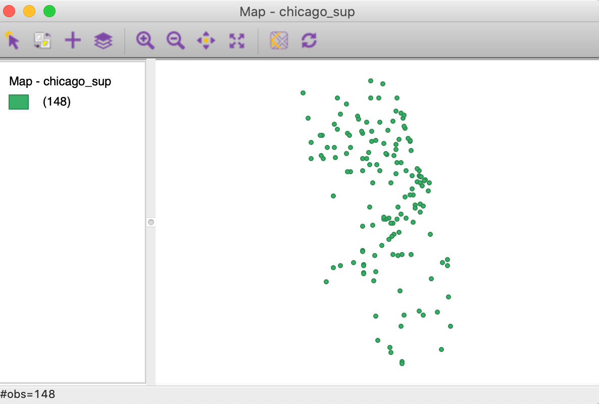
Figure 7: Themeless point map

Tabular files

In addition to GIS files, GeoDa can also read regular non-spatial tabular data. While this does not allow for spatial analysis (unless coordinates are contained in the table, see below), all non-spatial operations and graphs are supported.

For example, we can input a comma separated file (csv format) by dragging the file commpopulation.csv from the commpop sample data set onto the Drop files here box. This generates the dialog shown in Figure 8. Since a csv file is pure text, there is no information on the type of the variables. GeoDa tries to guess the type and lists the Data Type for each field, as well as a brief preview of the table. At this point, the type can be changed before the data are moved into the actual data table.

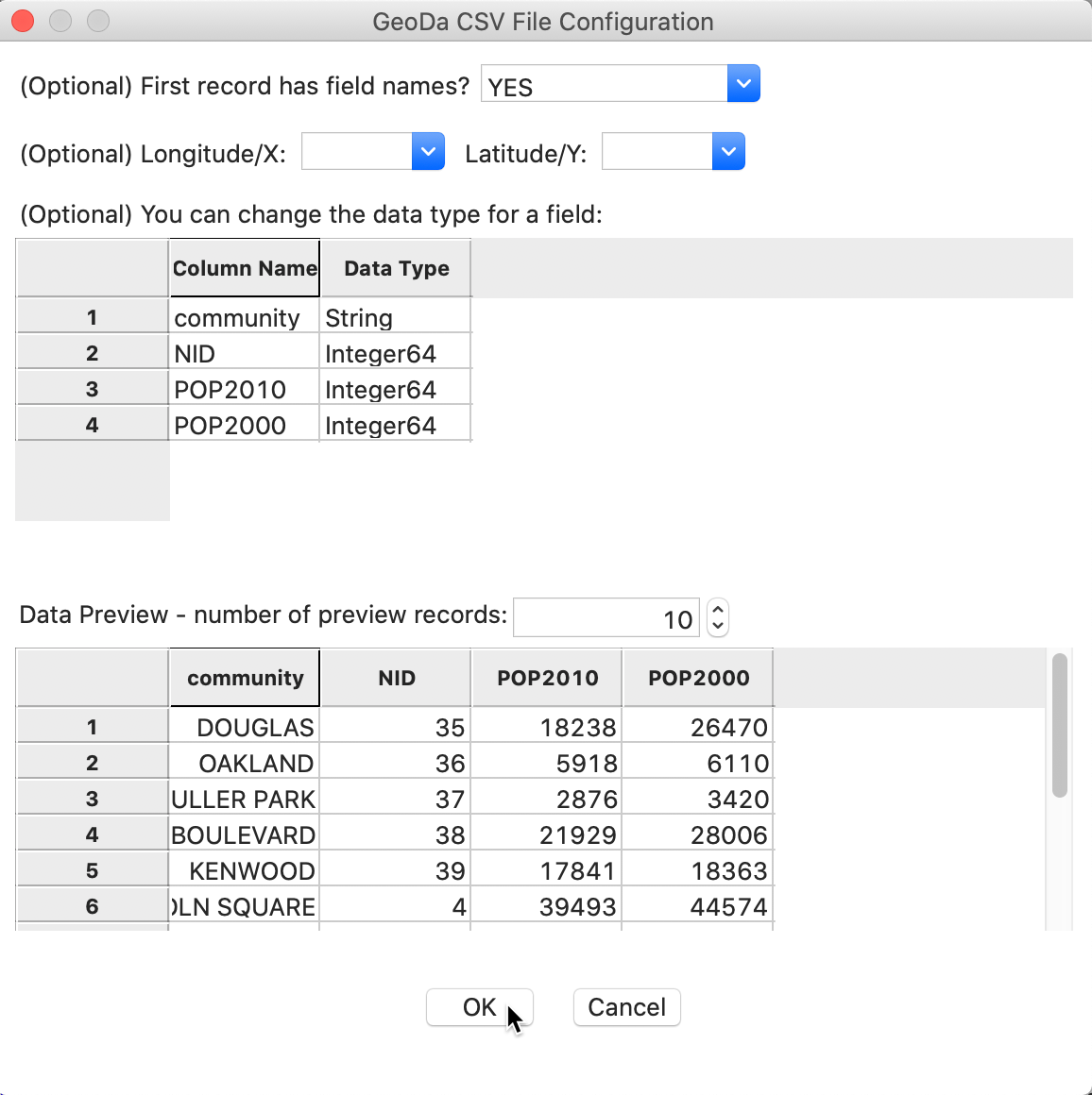
Figure 8: CSV format file input dialog

Instead of a base map, when the process is completed, the data table is brought up, as shown in Figure 9.

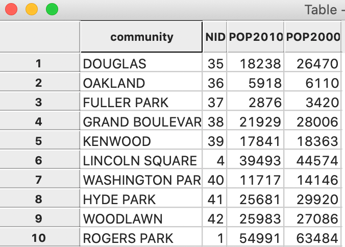
Figure 9: Table contents

In addition to comma separated files, GeoDa also supports tabular input from dBase database files, Microsoft Excel, and Open Document Spreadsheet (*.ods) formatted files.

Other spatial data input

In addition to file input, GeoDa can connect to a number of spatially enabled relational data bases, such as PostgesQL/PostGIS, Oracle Spatial and MySQL Spatial. This is available through the Database button in the Connect to Data Source interface, as shown in Figure 10. Each data base system has its own requirements in terms of specifying the host, port, user name, password and other settings. Once the connection is established, the data can also be saved to a file format. In the current version, the data base connection is limited to loading a single table, but it does not support additional SQL commands.

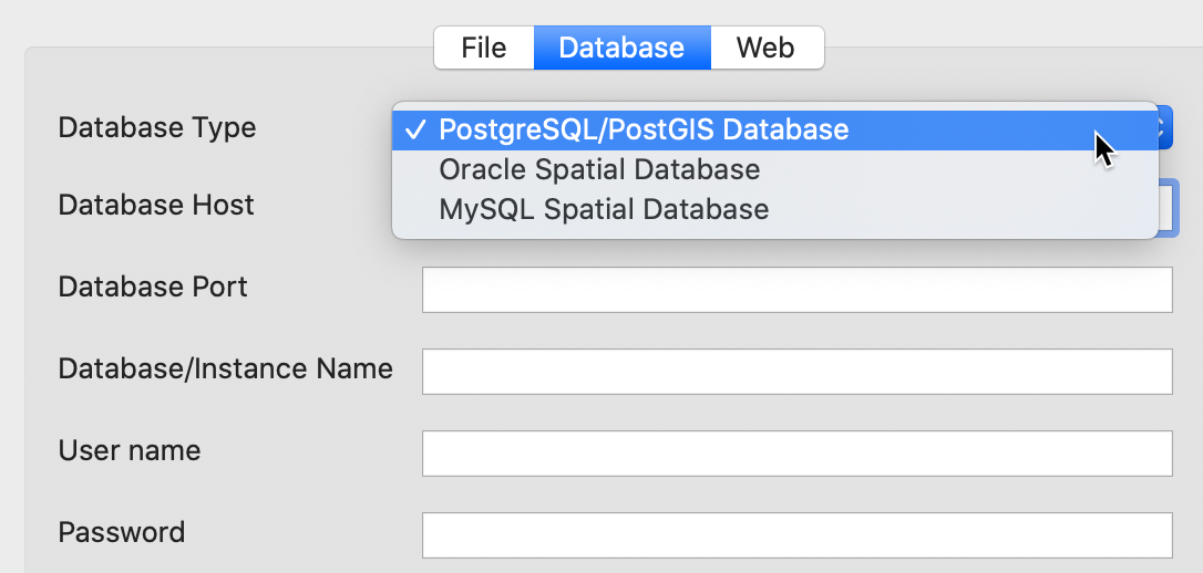
Figure 10: Spatial data base connections

A third data source option is referred to as Web in the interface. It allows data to be loaded directly from a GeoJSON URL or from the older web feature server WFS URL, as shown in Figure 11.

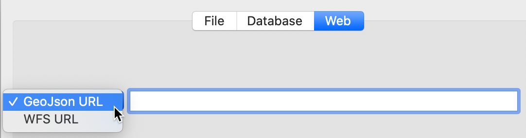
Figure 11: Web connections

Creating Spatial Layers

In addition to loading spatial layers from existing files or data base sources, the Tools functionality of GeoDa includes the capacity to create new spatial layers. This is invoked from the Tools icon on the toolbar, as in Figure 12, or from the menu as Tools > Shape. Two different operations are supported: one is to turn x-y coordinates from a table into a point layer, the other creates a rectangular shape of grid cells.

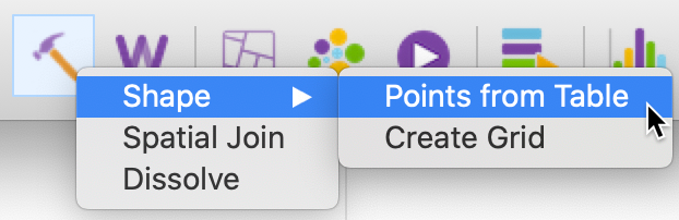
Figure 12: Tools Shape functions

Point layers from coordinates

Point layers can be created from two variables contained in a data table as Tools > Shape > Points from Table. To illustrate this, we first create a copy of chicago_sup.dbf from the grocery sample data set, say chicago_sup1.dbf. After loading the file onto the Drop files here box, the data table opens, as in Figure 13. The latitude and longitude of the points (in decimal degrees) are included as Ycoord and Xcoord. Note that latitude is the vertical dimension (Y) and longitude is the horizontal one (X).

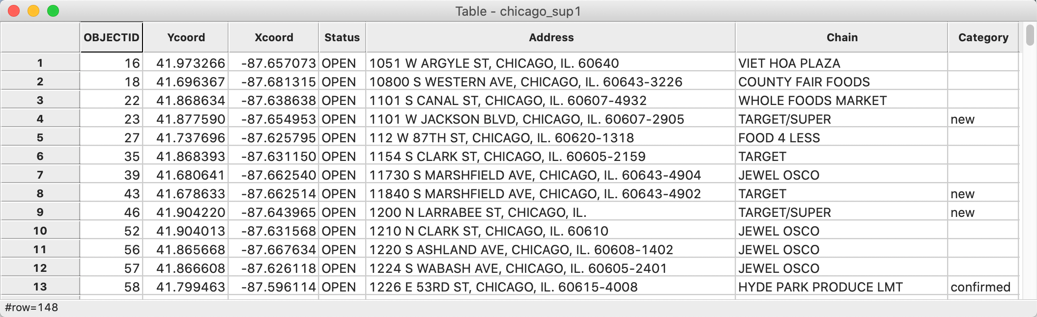
Figure 13: Coordinate variables in data table

At this point, we invoke the Points from Table command. A dialog opens up listing all numerical variables in the data table. In our example, shown in Figure 14, there are very few such variables, and the obvious candidates are Xcoord and Ycoord.

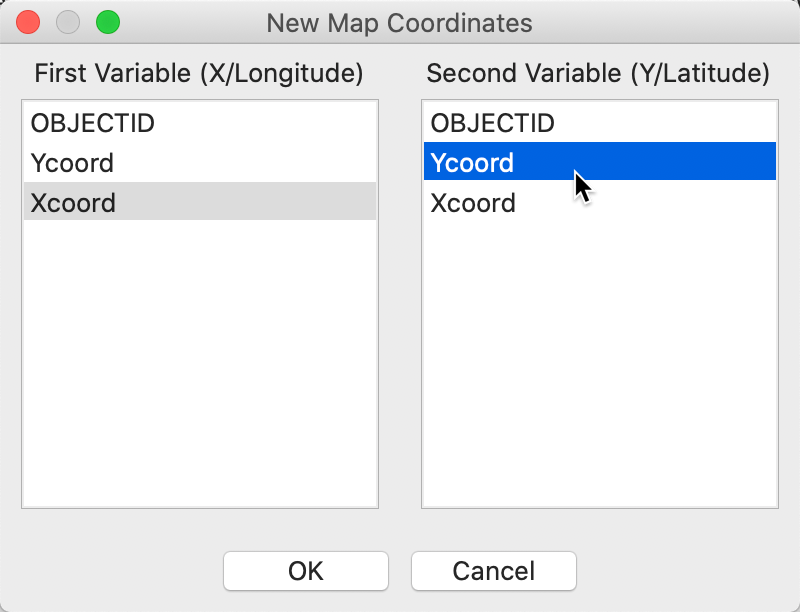
Figure 14: Specifying the point coordinates

After selecting the coordinate variables and clicking on OK, a point map appears, as in Figure 15.

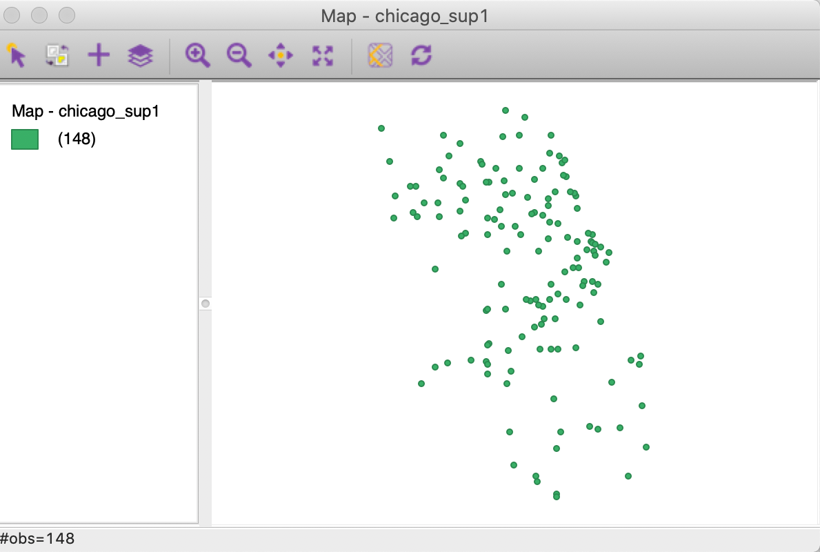
Figure 15: Point layer from coordinates

At this stage, we can save the point layer as a GIS file, such as a shape file, using File > Save As.

A first note about projections

At the bottom of the file dialog is an option to enter CRS (proj4 format). This refers to the projection information. We will discuss projections in more detail in the next chapter, but at this point it is useful to be aware of the implications.

A careful comparison of the point pattern in Figure 15 and in Figure 7 will reveal that they are not identical. While the relative positions of the points are the same, they appear more spread out in Figure 15. The reason for the discrepancy is in the use of different projections.

If, as described, a copy of the initial dbf file was used to create the point layer, then the Coordinate Reference System (CRS) entry will be empty, as in Figure 16. In other words, there is no projection information. As a result, if the result was saved as a shape file, it will not include a prj file.

Figure 16: Blank CRS

In contrast, if we had used the original chicago_sup.dbf file, the CRS box would contain the entry as in Figure 17. The reason for this difference is that GeoDa checks for the existence of a prj file with the same file name. If there is such a file present (as is the case in our sample data set), the information is used to populate the CRS entry, which then is saved into a prj file associated with the new point layer. We pursue this in greater detail in the next chapter.

Figure 17: CRS with projection information

Grid

The second type of spatial layer that can be created is a set of grid cells. Such cells are rarely of interest in and of themselves, but are useful to aggregate counts of point locations in order to calculate point pattern statistics, such as quadrat counts.

The grid creation can be invoked from the menu without any table or layer open, as Tools > Shape > Create Grid. This brings up a dialog containing a range of options, shown in Figure 18. The most important aspect to enter is the Number of Rows and the Number of Columns, listed under Grid Size at the bottom of the dialog. This determines the number of observations. In our example, we have entered 10 rows and 5 columns, for 50 observations.

There are four options to determine the Grid Bounding Box, i.e., the rectangular extent of the grids. The most likely approach is to use the bounding box of a currently open layer or of an available shape data source. The Lower-left and Upper-right corners of the bounding box can also be set manually, or read from an ASCII file.

In our example in Figure 18, we have selected the commpop shape file as the source for the bounding box.

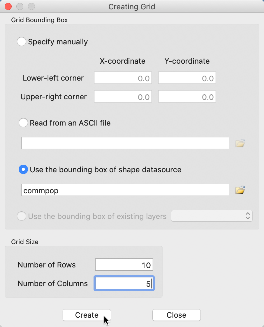
Figure 18: Grid creation dialog

After the grid layer is saved, it can be loaded into GeoDa. In Figure 19, the result is shown, superimposed onto the community areas layer (we will cover in the next chapter how to implement this). Clearly, the extent of the grid cells matches the bounding box for the area layer.

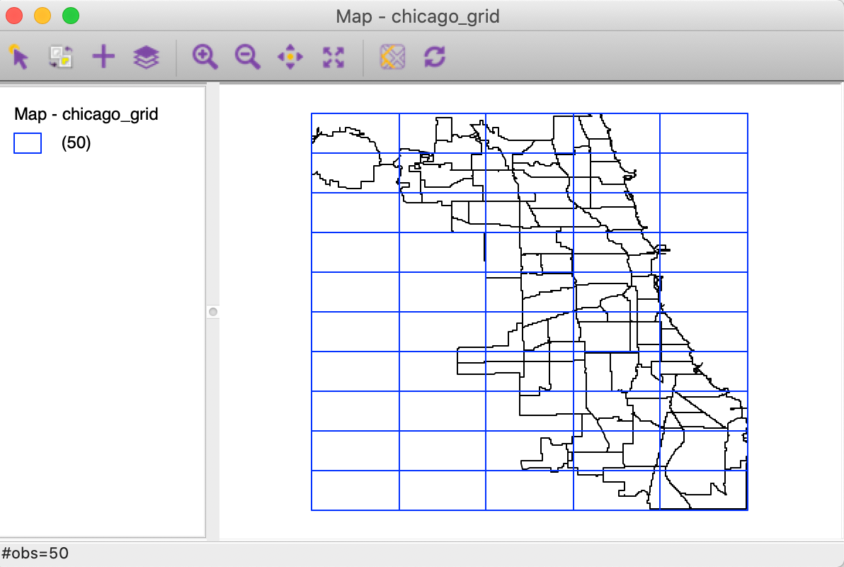
Figure 19: Grid layer over Chicago community areas

Table Manipulations

A range of variable transformations are supported through the Table functionality in GeoDa. To illustrate these, we will use the Natregimes sample data set. After loading the natregimes.shp file, we obtain the base map of 3085 U.S. counties, shown in Figure 20.

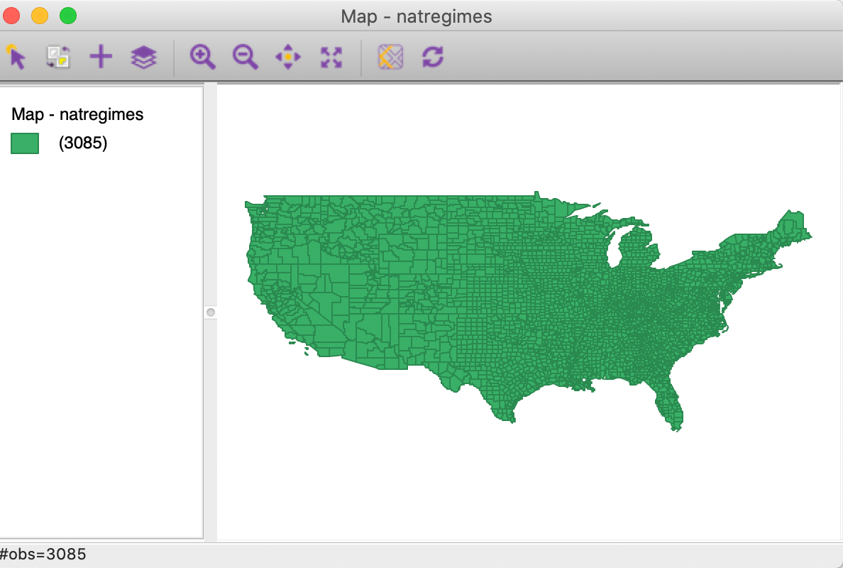
Figure 20: U.S counties base map

The table is openened by means of second icon from right on the toolbar shown in Figure 1, or from the menu. The data table associated with the natregimes layer is as in Figure 21.

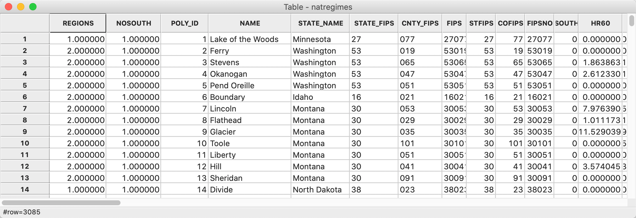
Figure 21: U.S counties data table

The options associated with table manipulations are invoked from the menu, or by right clicking on the table itself, as in Figure 22. In addition to a range of variable transformations, the options menu also includes the Selection Tool to carry out data queries. We discuss those options in the next section, first we review some of the more often used variable manipulations.

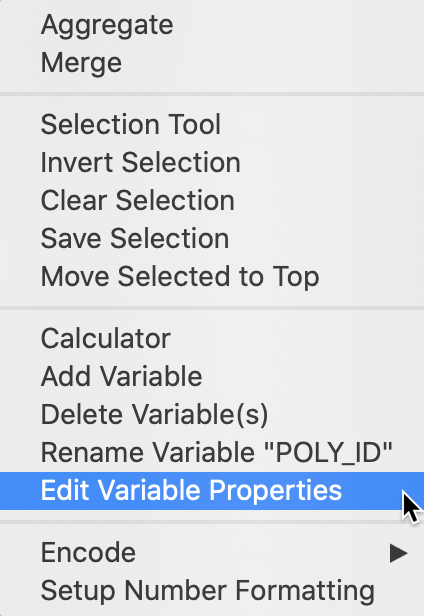
Figure 22: Table options

Variable properties

Edit variable properties

One of the most used initial transformations pertains to getting the data into the right format. Often, observation identifiers, such as the FIPS code used by the U.S. census, are recorded as character or string variables, not in a numeric format. In order to use these variables effectively, we need to convert them to a different format. This is accomplished through the Edit Variable Properties option.

After this option is invoked, a list of all variables is given, with their type, as well as a number of other properties, like precision, as shown in Figure 23. In our example, the indicator variable NOSOUTH is listed as real, whereas it really should be integer. By selecting the proper format from the drop down list, the change is immediate. As mentioned, the most common use of this functionality is to change string variables to a numeric format.

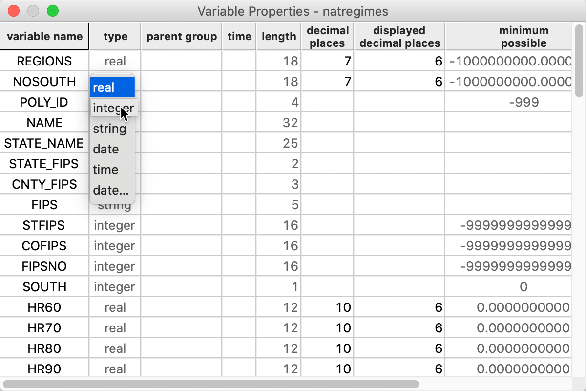
Figure 23: Edit variable properties

Other variable operations

The other variable operations listed in the drop down list in Figure 22 are mostly self-explanatory. For example, a new variable can be included through Add Variable (its value is obtained through the Calculator, see next), or variables can be removed by means of Delete Variable(s). Rename Variable operates on a specific column, which needs to be selected first.

Two more obscure options are Encode and Setup Number Formatting. The default encoding in GeoDa is Unicode (UTF-8), but a range of other encodings that support non-western characters are available as well. The default numeric formatting is to use a period for decimals and to separate thousands by a comma, but the reverse can be specified as well, which is common in Europe.

Operating on the table

The columns, rows and cells of the table can be manipulated directly, similar to spreadsheet operations. For example, the values in a column can be sorted in increasing or decreasing order by clicking on the variable name. A > or < sign appears next to the variable name to indicate the sorting order. The original order can be restored by sorting on the row numbers (the left-most column).

Individual cell values can be edited by selecting the cell and entering a new value. Such changes are only permanent after the table is saved. This is easily accomplished by clicking on the Save icon on the toolbar, i.e., the middle icon in Figure 1. Alternatively File > Save can be invoked from the menu.

Specific observations can be selected by clicking on their row number. The corresponding entries will be highlighted in yellow. Additional observations can be added to the selection in the usual way, by means of shift-click or command-click. The selected observations can be located at the top of the table by means of Move Selected to Top.

Finally, the arrangement of the columns in the table can be altered by dragging the variable name and moving it to a different position. This is often handy to move related variables next to each other in the table for easy comparison (for an illustration, see Figure 32).

Calculator

To illustrate the Calculator functionality, we return to the Chicago community area sample data and load the commpopulation.csv file. This file only contains the population totals, as shown in Figure 9.

The Calculator interface is shown in Figure 24. It contains six tabs, dealing, respectively, with Special functions, Univariate and Bivariate operations, Spatial Lag, Rates and Date/Time. Spatial Lag and Rates are advanced functions that are discussed separately in later chapters.

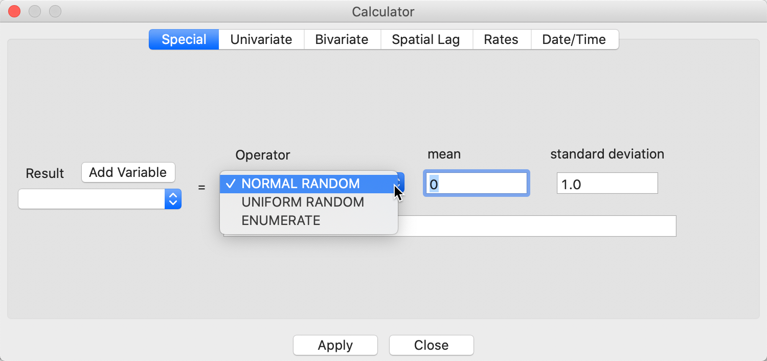
Figure 24: Calculator interface

Each operation begins by identifying a target variable in which the result of the operation will be stored. Typically, this will be a new variable, which is created by means of the Add Variable button. For example, in Figure 25, the dialog is shown for a new variable POPCH that we will use below to illustrate bivariate operations.

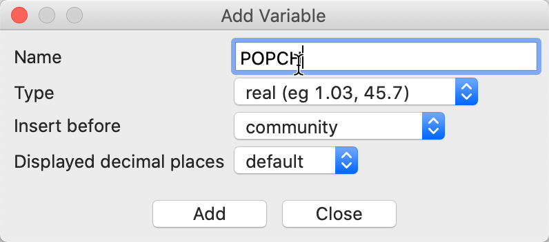
Figure 25: Add Variable interface

The Type of the variable can be specified, as well as its precision and where to insert it into the table. The default is to place a new variable to the left of the first column in the table, but any other variable can be taken as a reference point. In addition, the new variable can be placed at the right most end of the table.

Special

The three Special functions are shown in the drop down list in Figure 24. Both NORMAL and UNIFORM RANDOM variables can be created. The ENUMERATE function is somewhat unique. It creates a variable with the current order of the observations. This is especially useful to retain the order of observations after sorting on a given variable.

Univariate

Operations that pertain to a single variable are included in the Univariate drop down list, shown in Figure 26. The first six operations are straightforward transformations, such as changing the sign, taking the inverse or the square root, or carrying out a log transformation. ASSIGN allows a variable to be set equal to any other variable, or to a constant (the typical use).

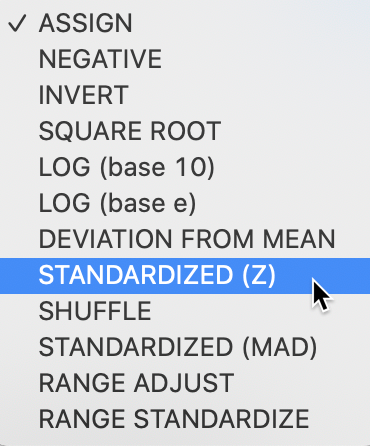
Figure 26: Univariate operations

SHUFFLE randomly permutes the values for a given variable to different observations. This is an efficient way to implement spatial randomness, i.e., an allocation of values to locations, but where the location itself does not matter (any location is equally likely to receive a given observation value).

Variable standardization

The univariate operations also include five types of variable standardization. The most commonly used is undoubtedly STANDARDIZED (Z). This converts the specified variable such that its mean is zero and variance one, i.e., it creates a z-value as \[z = \frac{(x - \bar{x})}{\sigma(x)},\] with \(\bar{x}\) as the mean of the original variable \(x\), and \(\sigma(x)\) as its standard deviation.

A subset of this standardization is DEVIATION FROM MEAN, which only computes the numerator of the z-transformation.

An alternative standardization is STANDARDIZED (MAD), which uses the mean absolute deviation (MAD) as the denominator in the standardization. This is preferred in some of the clustering literature, since it diminishes the effect of outliers on the standard deviation (see, for example, the illustration in Kaufman and Rousseeuw 2005, 8–9). The mean absolute deviation for a variable \(x\) is computed as: \[\mbox{mad} = (1/n) \sum_i |x_i - \bar{x}|,\] i.e., the average of the absolute deviations between an observation and the mean for that variable. The estimate for \(\mbox{mad}\) takes the place of \(\sigma(x)\) in the denominator of the standardization expression.

Two additional transformations that are based on the range of the observations, i.e., the difference between the maximum and minimum. These the RANGE ADJUST and the RANGE STANDARDIZE options.

RANGE ADJUST divides each value by the range of observations: \[r_a = \frac{x_i}{x_{max} - x_{min}}.\] While RANGE ADJUST simply rescales observations in function of their range, RANGE STANDARDIZE turns them into a value between zero (for the minimum) and one (for the maximum): \[r_s = \frac{x_i - x_{min}}{x_{max} - x_{min}}.\] Note that any standardization is limited to one variable at a time, which is not very efficient. However, most analyses where variable standardization is recommended, such as in the multivariate clustering techniques, include a transformation option that can be applied to all the variables in the analysis simultaneously. The same five options as discussed here are available to each analysis.

Bivariate

The bivariate functionality includes all classic algebraic operations. The target variable is selected from the drop down list on the left in Figure 27. Then the respective variables (or a constant) are entered in the dialog with the appropriate operation taken from the drop down list. In the example in Figure 27, we compute the population change for the Chicago community areas between 2010 and 2000. The result is added to the table, but is only permanent afer a Save operation.

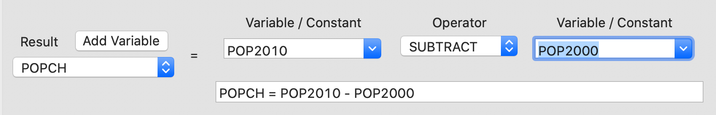
Figure 27: Example bivariate operations

Date and time

The calculator also contains limited functionality to operate on date and time fields. In practice, this can be quite challenging, due to the proliferation of formats used to define variables pertaining to dates and time. To illustrate these operations, we will use the SanFran Crime data set from the sample collection, which is one of the few sample data sets that contains a date stamp.

We load the sf_cartheft.shp shape file from the Crime Events subdirectory of the sample data set. This data set contains the locations of 3384 car thefts in San Francisco between July and December 2012. After loading the data, the point layer base map appears, as in Figure 28.

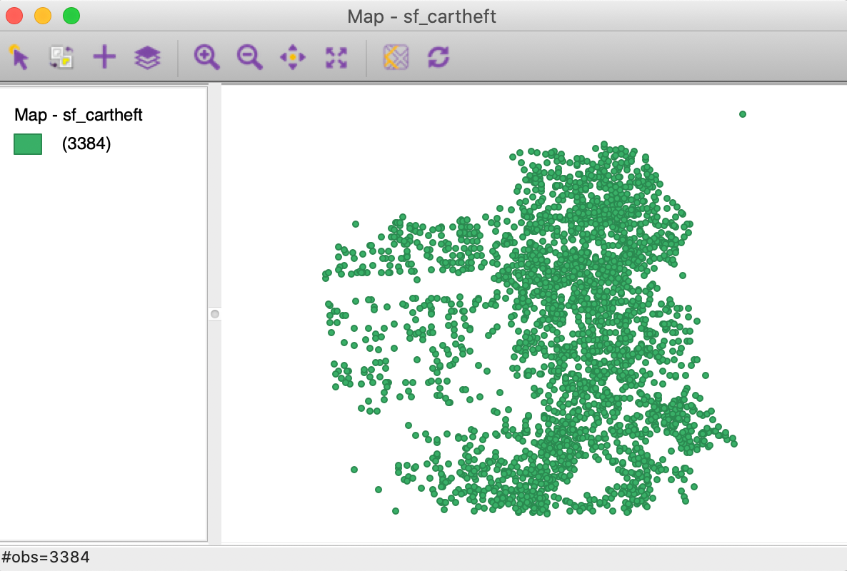
Figure 28: San Francisco car theft point map

We bring up the data table and note the variable Date in the seventh column in Figure 29.

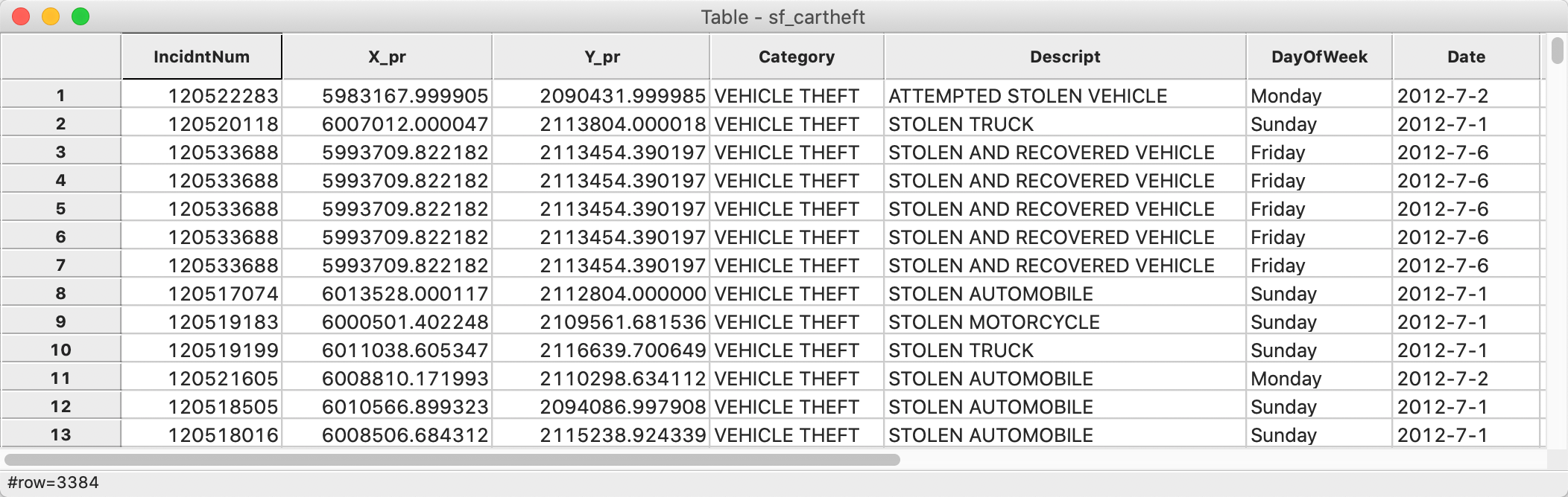
Figure 29: San Francisco car theft table

At first sight, it seems like the date is formatted as a string, since it is left-aligned. However, when we examine the type by means of the Edit Properties function, we see that it is indeed in the date format, as shown in Figure 30.

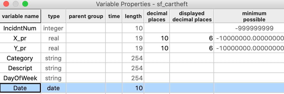
Figure 30: Variable property of Date

The date format supports a number of functions to extract components of the date as integers. This is often necessary, because the date type currently cannot be used in queries. For example, in Figure 31, the operator Get Month turns the month that is contained in the Date variable into an integer, assigned to the new variable Month.

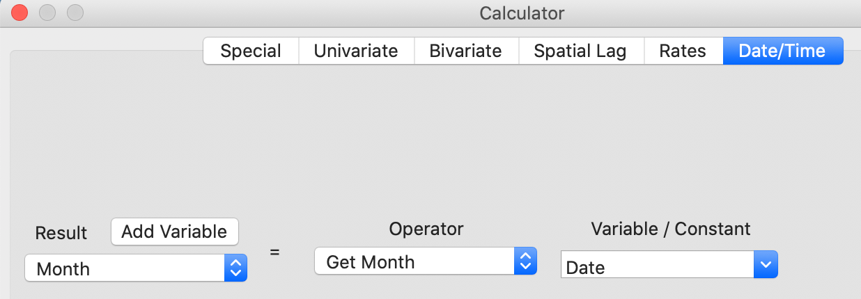
Figure 31: Get Month in Calculator

As shown in Figure 32 (after moving the columns around to put the original date next to the new variable), the transition from dates in July to August is reflected in the Month variable changing from 7 to 8.

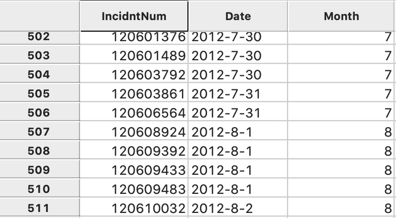
Figure 32: Extracted month in table

Merging tables

An important operation on tables is the ability to Merge new variables into an existing data set. We illustrate this with the Chicago community area population data and load commpop.shp. We also bring up the data table and select Merge from the options. The resulting dialog is as in Figure 33.

A number of important parameters need to be selected. First is the datasource from which the data will be merged. In our example, we have chosen commpopulation.csv. Even though this contains the same information as we already have, we select it to illustrate the principles behind the merging operation.

We click on the open file icon and use the standard procedure to load the csv file. After this, the file name commpopulation is listed as the data source. The default method is Merge, but Stack is supported as well. The latter operation is used to add observations to an existing data set.

Best practice to carry out a merging operation is to select a key, i.e., a variable that contains (numeric) values that match the observations in both data sets. Using a key is superior to merging by record order, since there is often no guarantee that the actual ordering of the data in the two sets is the same, even though it may seem so in the interface (such as the table view). In our example, we select NID as the key in both data sets.

Finally, we need to decide which variables will be merged. Here, we used the >> key to move all variables from the Exclude box to the Include box.

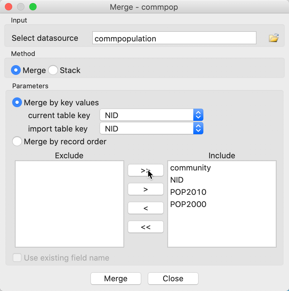
Figure 33: Merge dialog

Upon clicking Merge, the new variables will be added to the data table, unless there is a potential conflict of variable names. This conflict can be two-fold. First, when variables have identical names in both data sets, they need to be differentiated. Clearly, this is the case here, as shown in Figure 34, where alternatives are suggested. These alternatives are not always the most intuitive and can be readily edited in the entry box. A second potential conflict is when the variable name has more than 10 characters. In csv input files, there are no constraints on variable name length, but the dbf format used for the attribute values in a shape file format has a limit of 10 characters for a variable name. Again, an alternative will be suggested in the dialog, but it can be easily edited (as long as it stays within the 10 character limit).

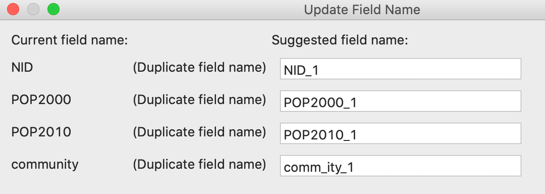
Figure 34: Update the names of the variables to be merged

The merged tables are as in Figure 35. We can verify that the correct observations line up. As before, the merger only becomes permanent after a Save operation.

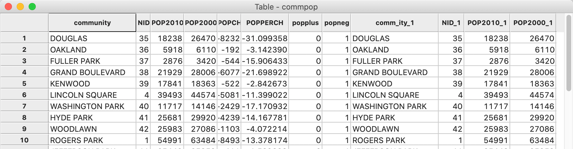
Figure 35: Merged tables

Queries

While queries of the data are somewhat distinct from data wrangling per se, drilling down the data is often an important part of selecting the right subset of variables and observations. We have already seen how we can remove variables from the data table by using the Delete function. In order to select particular observations or rows in the data table, we need the Selection Tool. The latter is arguably one of the most important features of the table options.

We will illustrate queries with the San Francisco car theft example and load the sf_cartheft shape file. We assume that the integer variable Month has been added to the table. If not, use the steps in the previous section to accomplish this.

Table Selection

With the data loaded and the table open, we choose Selection Tool from the options. The interface, shown in Figure 36, has several options and it supports quite complex searches, even though it may seem somewhat rudimentary.

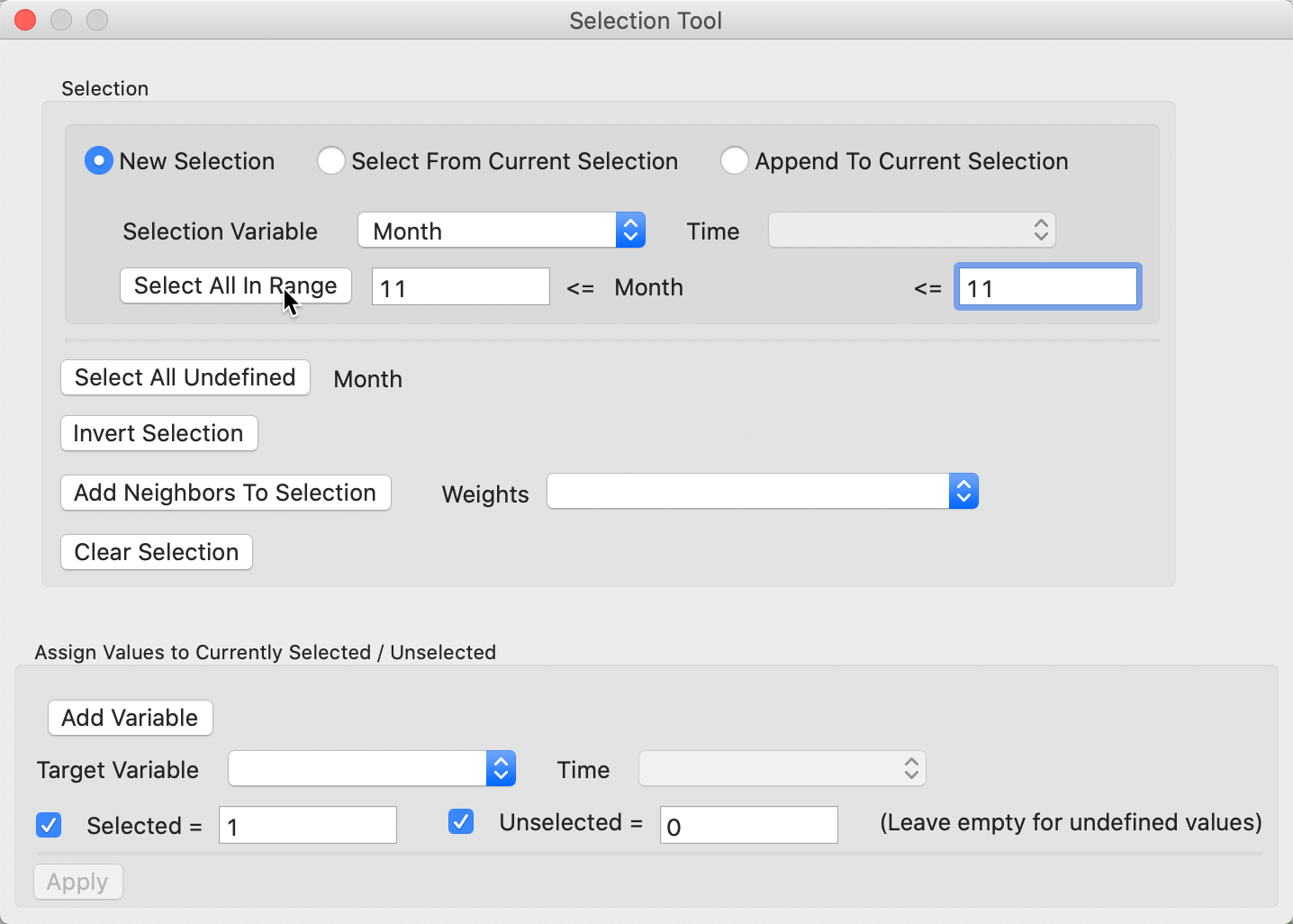
Figure 36: Selection Tool

New selection

The main panel of the interface deals with the selection criteria. In our example, we start a New Selection, as indicated by the radio button in the top line. We want to select the car thefts that occurred in the month of November. To that end, we specify the just created variable Month as the Selection Variable. Since we want the observations with Month = 11, we set the beginning and end value of the Select All in Range option to 11. Clicking on this button will select the observations that meet the selection criterion.

As we have already seen, the selected observations are highlighted in the table (and can be moved to the top of the table). They are also highlighted in the themeless point map, or rather, they retain their original shading, while unselected observations become transparent. This is illustrated in Figure 37. The status bar lists that 568 observations have been selected. In addition, the selected observations are also immediately highlighted in any other open graph or map. This is the implementation of linking, which will be discussed in more detail in a later chapter.

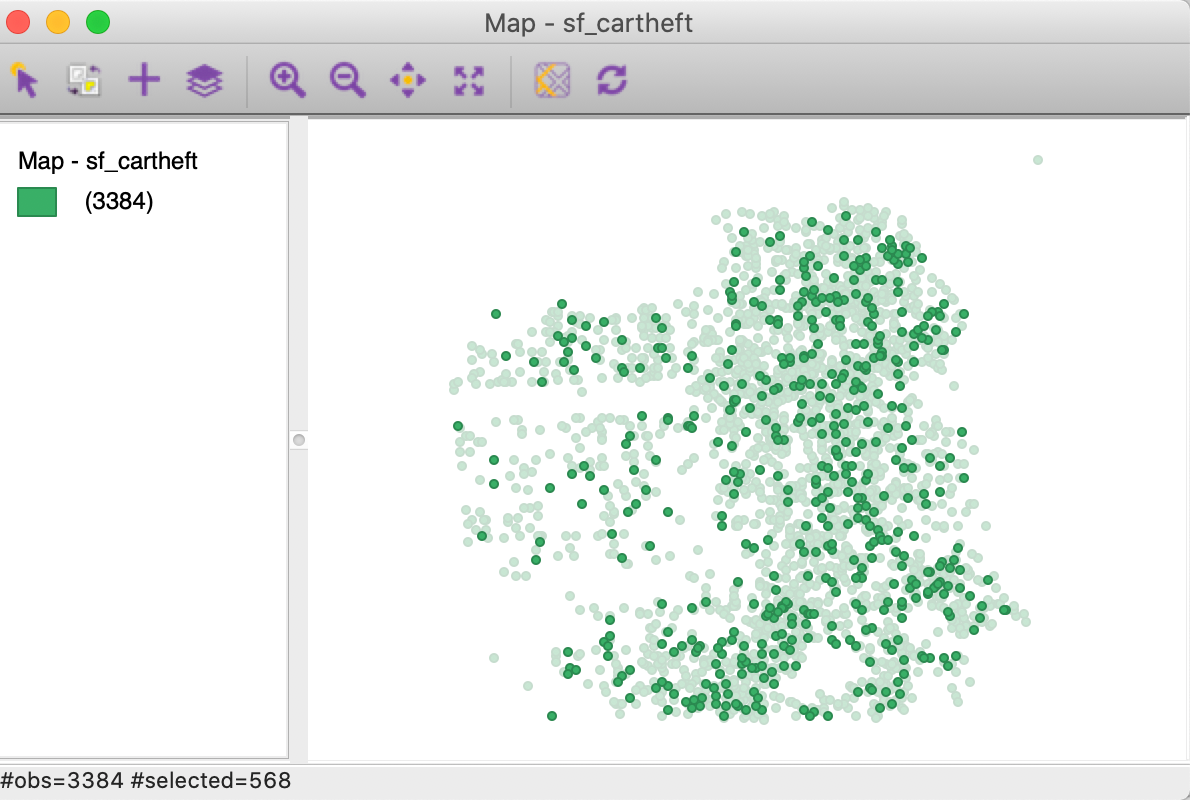
Figure 37: Selected observations in themeless map

Other selection options

The Selection Tool contains several more options to refine a selection. For example, a second criterion can be chosen to Select From Current Selection. For example, this would be the case if we wanted to select a particular day of the month of November (provided we created the corresponding integer variable). Alternatively, we could Append To Current Selection, say if we wanted both November and December.

A useful feature is to use Invert Selection to choose all observations except the selected ones. For example, we could use this to choose all months but November. This is often the most practical way to remove unwanted observations. First, we select them, and then we invert the selection, at which point we can Save Selected As (see below). This option is often used in combination with Select All Undefined, which identifies the observations with missing values for a given variable. After selecting them, we invert the selection and save this as a data set without missing values.

We will discuss Add Neighbors To Selection in the chapters dealing with spatial weights.

Indicator variable

Once observations are selected in the table, a new indicator variable can be created that typically holds the value of 1 for the selected observations, and 0 for the others, as shown in the bottom panel of Figure 36. However, any value can be specified in the dialog.

With a Target Variable specified, clicking on Apply will add the 0-1 values to the table.

Save selected observations

Arguably one of the most useful features of the selection tool in terms of data wrangling, is the ability to save the selected observations as a new data set. In our example, we chose File > Save Selected As and specify a new file name to save just the observations for November, say cartheftsNov. If we close the project and load the new file, the themeless map is as in Figure 38. Note how the point pattern has the same shape as the selected observations in Figure 37, but the number of observations is now listed as 568.

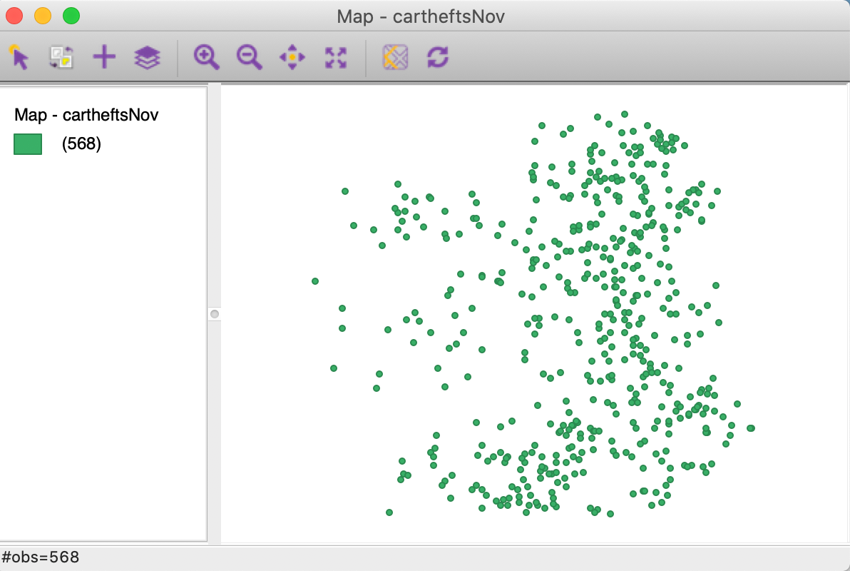
Figure 38: Selected observations in new map

Spatial selection

So far, we have carried out all selections through the Selection Tool in the Table. However, observations can also be selected visually from any map. To illustrate this, we bring back the sf_cartheft shape file (with the Month variable).

Even though a discussion of the mapping functionality in GeoDa is beyond the scope of the current chapter, we will first create a simple map of the points classified by month. To accomplish this, select Map > Unique Values Map from the menu, and chose the variable Month. The resulting map is as in Figure 39, with a different color associated with each month.

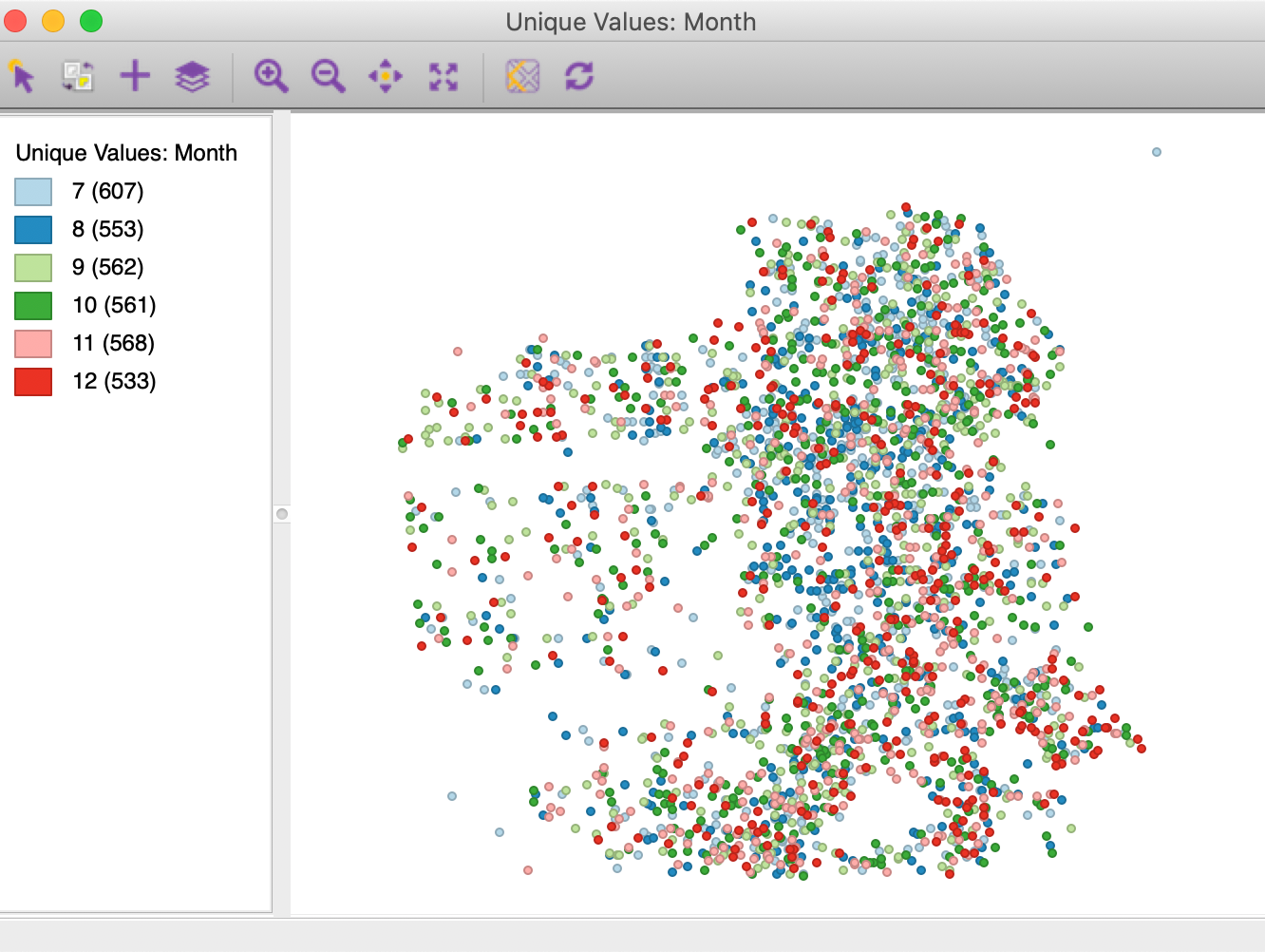
Figure 39: Car thefts by month

Selection by shape

The map selection tool is the default interaction with a map view. It can also be designated explicitly by clicking on the left-most icon in the map view toolbar (the arrow symbol).

Observations are selected by clicking on them or by drawing a selection shape around the target area. The default selection shape is a Rectangle, as in Figure 40, but Circle and Line are available as well. The particular shape is chosen by selecting Selection Shape from the map options menu (right click on the map).

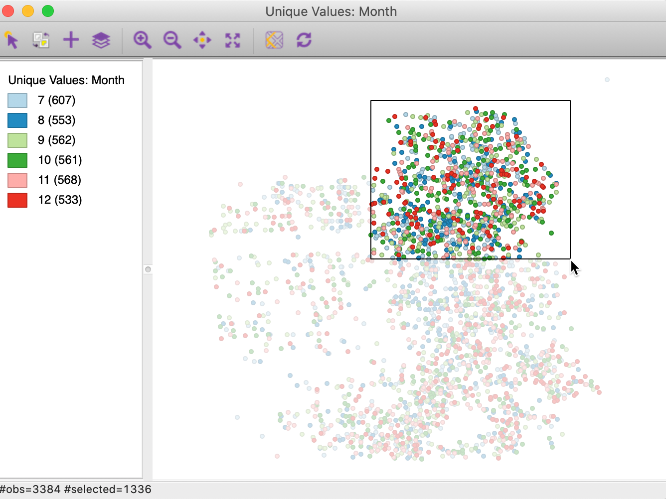
Figure 40: Selection on the map

Identical to table selection, all selected observations are highlighted in the table in yellow and in any other open map or graph (through linking). Also, they can be saved to a new data set using File > Save Selected As, in the same way as for a table selection.

The selection can be inverted by clicking on the second left-most icon in the map toolbar. This works in the same way as for table selection.

Selection on map classification

In addition to using a selection shape on a map, observations that fall into a particular map classification category can be selected by clicking on the corresponding legend icon. We discuss map classifications in a later chapter, but in Figure 41, we can see how the observations for the month November are selected by clicking on the small rectangle next to 11. The selected points match the pattern in Figure 37.

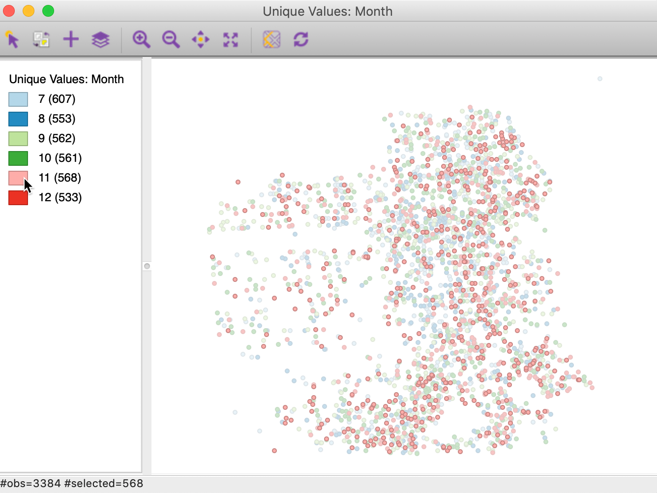
Figure 41: Selection on a map category

Save selection indicator variable

Finally, as is the case for a table selection, a new indicator variables can be saved to the table, with, by default, a value of 1 for the selected observations, and 0 for the others. This is invoked from the map options (right click on the map) by selecting Save Selection. The dialog shown in Figure 42 appears, with the default variables name of SELECTED.

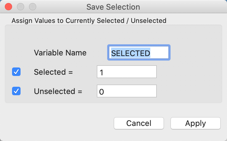
Figure 42: Selection variable dialog

As before, the variable name can be changed, as can the values assigned to selected and unselected. After the indictor variable is added to the table, it must be made permanent through a Save command.

References

Dasu, Tamraparni, and Theodore Johnson. 2003. Exploratory Data Mining and Data Cleaning. Hoboken, NJ: John Wiley & Sons.

Kaufman, L., and P. Rousseeuw. 2005. Finding Groups in Data: An Introduction to Cluster Analysis. New York, NY: John Wiley.

Rattenbury, Tye, Joseph M. Hellerstein, Jeffrey Heer, Sean Kandel, and Connor Carreras. 2017. Principles of Data Wrangling. Practical Techniques for Data Preparation. Sebastopol, CA: O’Reilly.

---

1. University of Chicago, Center for Spatial Data Science – anselin@uchicago.edu↩︎

GeoDa is maintained by lixun910. This page was generated by GitHub Pages using the Cayman theme by Jason Long.