Spatial Data Wrangling (3)

Introduction

In this lab, we will put into practice the data wrangling capability in GeoDa using a realistic example, illustrating a range of issues that may be encountered in practice. We will use the City of Chicago open data portal to download data on abandoned vehicles. Our end goal is to create a simple choropleth map that illustrates the spatial distribution of abandoned vehicles per capita for Chicago community areas in the month of April 2020.

In order to accomplish this, we will employ functionality outlined in more detail in the previous two chapters, to which we refer for specifics. However, this chapter can also be read on its own, since all required operations are explained in full.

Before we can create the maps, we will need to access the data source, select observations, aggregate data, join different files and carry out variable transformations in order to obtain a so-called spatially intensive variable (per capita abandoned vehicles) for mapping.

Objectives

Identify the necessary data and download from the proper source, such as any Socrata-driven open data portal, e.g., the City of Chicago open data portal
Create a data table from a csv formatted file
Manipulate variable formats, including date/time formats
Edit table entries
Create a new data layer from selected observations
Convert a table with point coordinates to a point layer in GeoDa
Changing the projection for a spatial layer
Spatial join
Spatial aggregation
Merge tables
Calculate new variables
Create a simple quantile map

GeoDa functions covered

File > Open
- data source connection dialog
- csv input file configuration
File > Save As
- specify CRS
File > Save Selected As
Table > Edit Variable Properties
Table edits
- Sort table on a variable
- Edit table cells
Table > Delete Variables
Table > Selection Tool
Table > Calculator
Table > Merge
Table > Aggregate
Tools > Shape > Points from Table
Tools > Spatial Join
Map > Quantile Map

Obtaining data from the Chicago Open Data Portal

Our first task is to find the information for abandoned vehicles on the data portal and download it to a file so that we can manipulate it in GeoDa. The format of choice is a comma delimited file, or csv file. This is basically a spreadsheet-like table with the variables as columns and the observations as rows.

Finding the information

We start by going to the City of Chicago open data portal. The first interface looks as in Figure 1:

Figure 1: City of Chicago Open Data Portal

The type of information we need is termed a Service Requests. Selecting this button yields a list of different types of 311 nuisance calls, as shown in Figure 2:

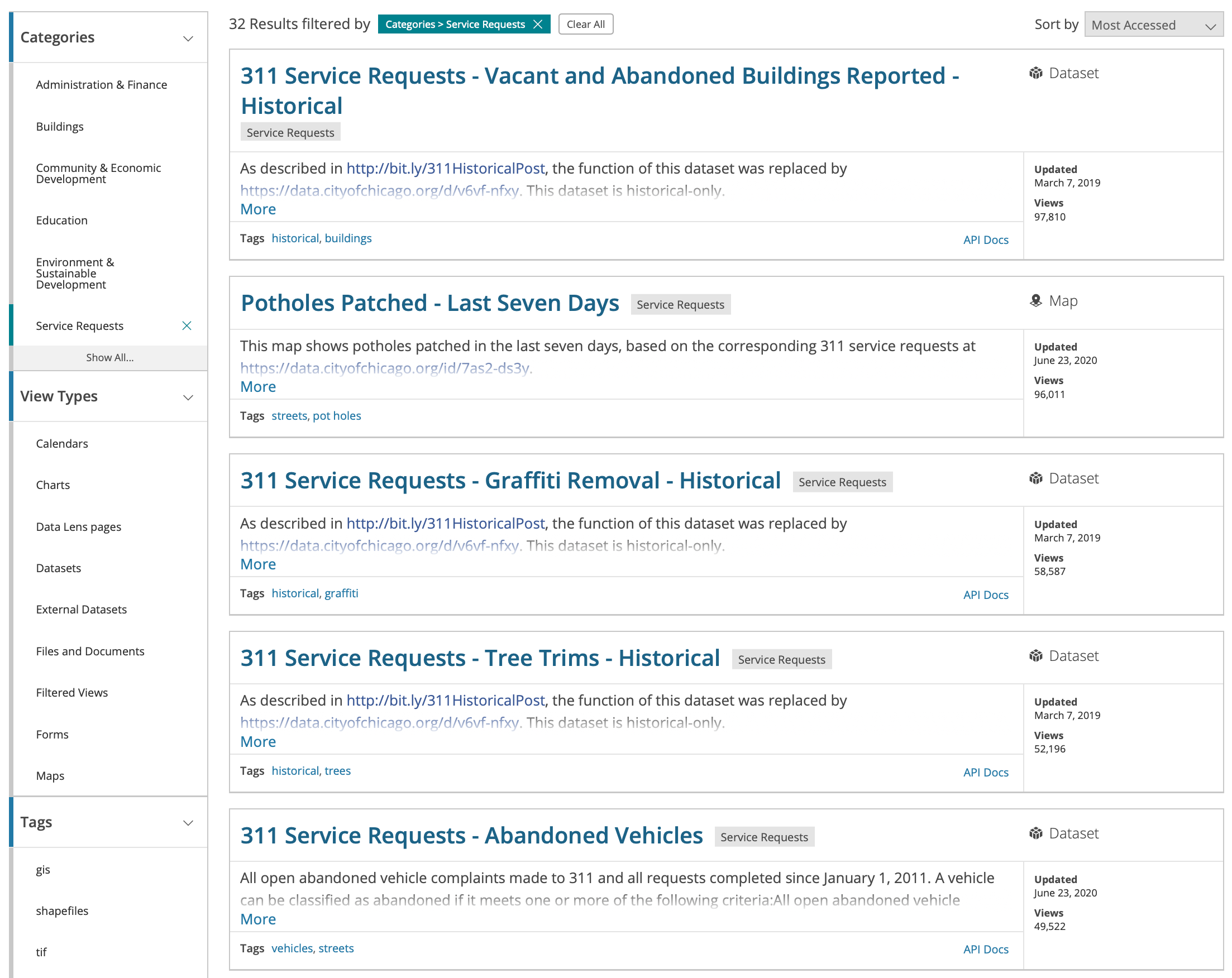
Figure 2: City of Chicago Service Requests

We select 311 Service Requests - Abandoned Vehicles. A brief description of the data source is provided, as shown in Figure 3:

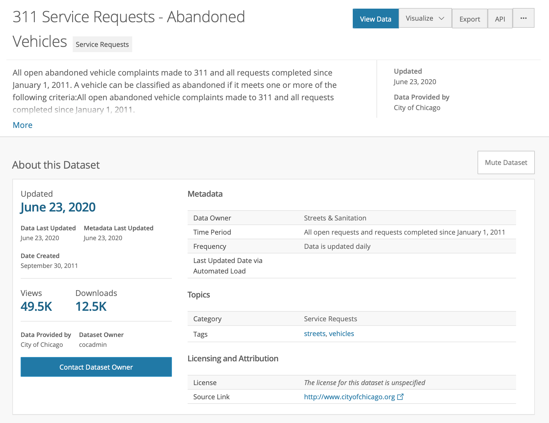
Figure 3: 311 Requests for Abandoned Vehicles

Your description may differ slightly, since the site is constantly updated. The figure above was created on June 23, 2020.

Below the summary is a list of all the variables (columns) contained in the data set, shown in Figure 4, as well as information on the data type (after clicking on the down arrow to the right).

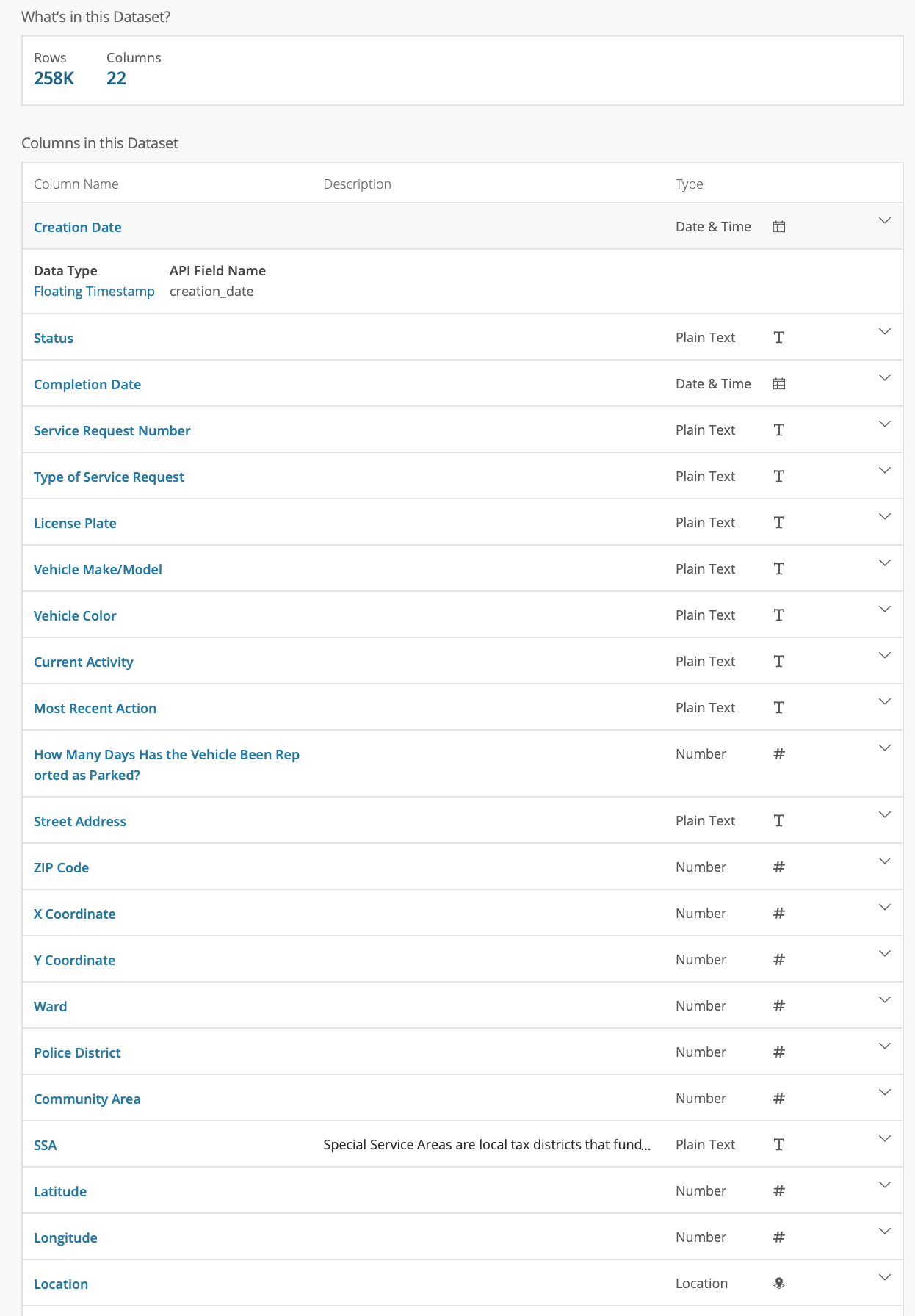
Figure 4: Abandoned Vehicles table content

Downloading the data

Note that this data table contains some 258,000 observations (as of June 23, 2020 – this will change over time). Below the summary of the variables, there is a snapshot of the table and there are some visualization options. We will not pursue those, but download the data as a comma separated (csv) file, by selecting the Export butten and clicking on CSV, as shown in Figure 5.

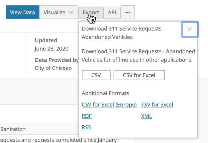
Figure 5: Download csv Format

The file will be downloaded to your drive. Note: this is a very large file (some 72 Mb) so it may take a while!

You can now open this file in a spreadsheet to take a look at its contents, or, alternatively, open it in a text editor, or use the linux head command to check out the top few lines. It is quite unwieldy and is not shown here. Inspecting the cells, you can identify many empty ones. In addition, the coding is not entirely consistent. We will deal with this by selecting only those variables/columns that we are interested in and only taking a subset of observations for a given time period, in order to keep things manageable.

Selecting Observations for a Given Time Period

For the sake of this exercise, we don’t want to deal with all observations. Instead, say we are interested in analyzing the abandoned vehicle locations for a given time period, such as the month of April 2020, in the middle of the COVID crisis in Chicago. To get to this point, we will need to move through the following steps:

import the csv file into GeoDa
convert the date stamp into the proper Date/Time format
extract the year and month from the date format
select those observations for the year and month we want
keep only those variables/columns of interest to us
create a new data set with the selected observations and variables

The end result of this process will be a data table saved in the legacy dBase (dbf) format.

Loading the data

The first step is to load the data from the csv file into GeoDa. After launchig GeoDa, the Connect to Data Source dialog should open. Next, we drag the file _311_Service_Requests_-_Abandoned_Vehicles.csv_ (or its equivalent, if you renamed the file) into the Drop files here box of the data dialog, as illustrated in the previous chapters. Since the csv format is a simple text file without any metadata, there is no way for GeoDa to know what type the variables are, or other such characteristics of the data set. To set some simple parameters, the CSV File Configuration dialog pops up, as in Figure 6.

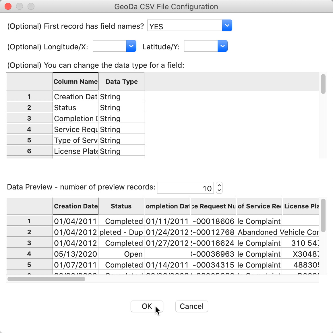
Figure 6: CSV File Configuration

The program tries to guess the type for the variables, but in this instance mostly treats them as String. We will deal with this later. For now, make sure the First record has field names item is set to YES (the default setting), and leave all other options as they are. After clicking the OK button, the data table will show the contents of the file, with the number of observations (258153) in the status bar at the bottom, as in Figure 7. For data sets downloaded other than on June 23, 2020, the number of observations will be different. However, since we limit the analysis to April 2020, those data will be the same, no matter when the full file is downloaded (unless the data for April were somehow updated at a later point in time).

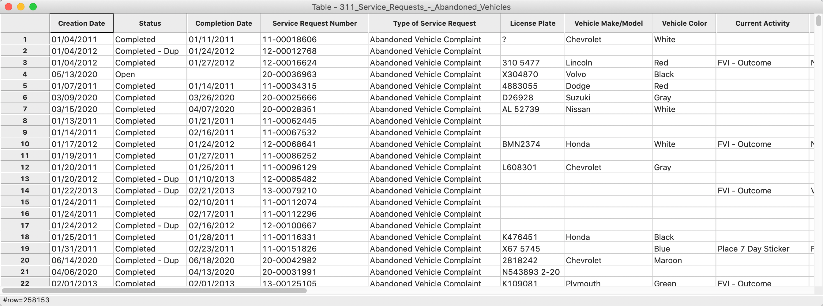
Figure 7: Table Contents

Note the many empty cells in the table, as well as some non-standard notation, such as the ? for the License Plate variable of the first observations. As is typically the case for public information downloaded from open data portals, the resulting files are far from clean and require quite a bit of pre-processing before they can be used for analysis. This is the 80% effort devoted to data wrangling that we referred to in the first chapter.

Converting a string to date format

We want to select the observations for the month of April in 2020. Before we can create the query, we need to transform the Creation Date to something manageable that we can search on. As it stands, the entries are in string format (sometimes also referred to as character format). We can check this by means of the Edit Variable Properties option in the Table menu, invoked either by right-clicking, or by selecting Table > Edit Variable Properties from the menu.

A cursory inspection of the type shows the Creation Date to be string. This is not what we want, so we click on the string item and select date from the drop down list, as in Figure 8.

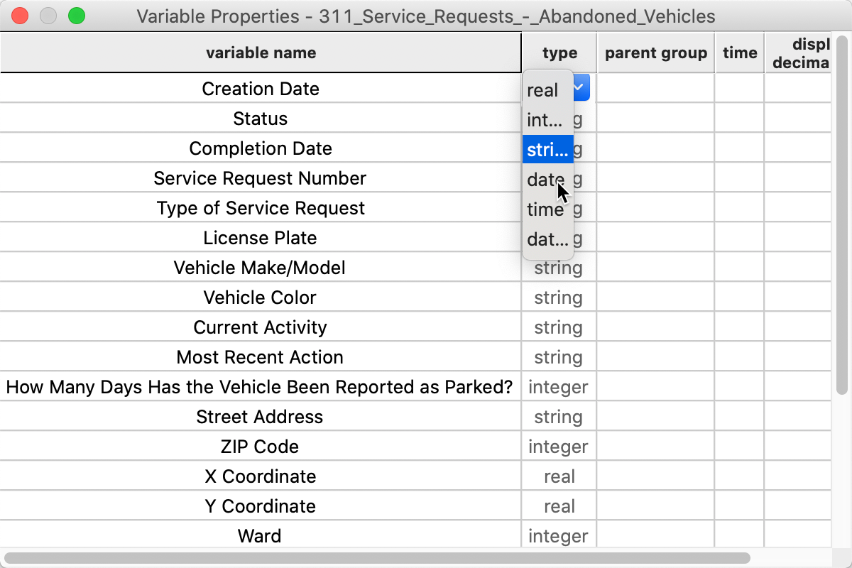
Figure 8: Changing the variable type to Date

GeoDa is able to recognize a range of date and time formats. The complete list is available from the Preferences dialog, using the Data Sources tab. If the data source contains a date or time format that is not included in the list, it can be added through the Preferences dialog, using the standard conventions to refer to year, month, day, etc.

In our example (there might be slight differences, depending on when the data were downloaded), the previous entry in the data table of 01/04/2011 for Creation Date in the first row is now replaced by a proper date format as 2011-04-11, as in Figure 9. Contrast this with the entry for Completion Date, which is still in the old format, as 01/11/2011.

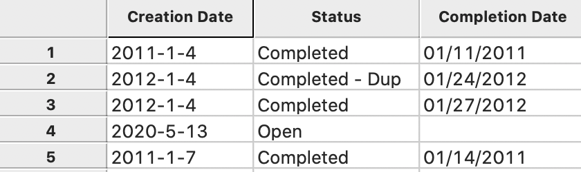
Figure 9: Creation Date in Table

Extracting the month and year from the creation date

Currently, search functionality on date formats is not implemented in GeoDa. However, we can extract the year and month as integer and then use those in the table Selection Tool. In order to get the year and month, we need to use the Calculator functionality in the table menu (Table > Calculator). or choose this item in the table option menu (right click in the table).

As we have seen in the previous chapters, the calculation of new or transformed variables operates in two steps:

add a new variable (place holder for the result) to the table
assign the result of a calculation to the new variable

The types of computations are listed as tabs at the top of the Calculator dialog. The right-most tab pertains to Date/Time. This allows us to manipulate the contents of a date/time object, such as extracting the month or the year.

We will use this tab to create new integer variables for the year and for the month. First, we select Add Variable to bring up a dialog to specify the properties of the new variable. For example, we can set year to be an integer variable. We can also specify where in the table we want the new column to appear. The default is to put it to the left of the first column, which we will use here. The new variables can also be added at the end of the columns, or inserted anywhere specified in front (i.e., to the left) of a given field.

After pressing the Add button, a new empty column will be added to the data table. Now, we go back to the Calculator dialog. We specify the new variable year as the outcome variable for the operation and select Get Year from the Operator drop down list. The Variable/Constant should be set to Creation Date, as in Figure 10.

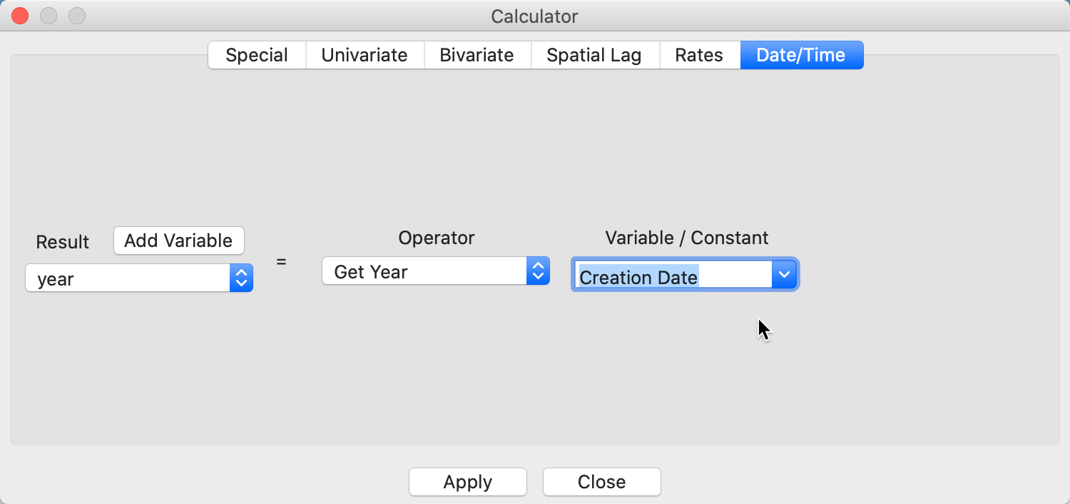
Figure 10: Extract Year

After clicking on Apply, an integer with the value for the year will be inserted in the year column of the table. We proceed in the same fashion to create a variable month and then use Get Month to extract it from the Creation Date. After these operations, there are two new columns in the data table, respectively containing the month and the year, as in Figure 11 (again, depending on when the original data were downloaded, the results may look slightly different).

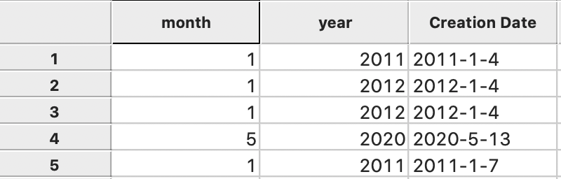
Figure 11: Month and Year in Data Table

Extracting observations for the desired time period

We now have all the elements in place to design some queries to select the observations for the month of April 2020 (or any other time period). We invoke the table Selection Tool from the main menu, as Table > Selection Tool, or from the options menu by right-clicking on the table. We proceed in two steps. First, we select the observations for the year 2020, then we select from that selection the observations for the month of April.

The first query is carried out with the New Selection radio button checked, and year as the Selection Variable. We specify the year by entering 2020 in both boxes for the <= conditions. Then we click on Select All in Range, as in Figure 12. The selected observations will be highlighted in yellow in the table (since this is a large file, you may not see any yellow observations in the current table view – the selected observations can be brought to the top by choosing Move Selected to Top from the table menu, or by right clicking in the table and selecting this option). The number of selected observations will be listed in the status bar. In this example, there were 13,237 abandoned vehicles in Chicago in 2020 as of June 23 (results may be slightly different, depending on the download date).

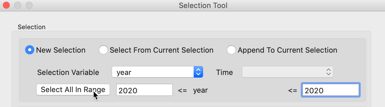
Figure 12: Select Year

For the second query, we check the radio button for Select From Current Selection and now specify month as the Selection Variable. We enter 4 in the selection bounds boxes and again click on Select All in Range, as in Figure 13. The selected observations will now be limited to those in 2020 and in the month of April. Again, the corresponding lines in the table will be highlighted in yellow, and the size of the selection given in the status bar. In this case, there were 1,383 abandoned vehicles.

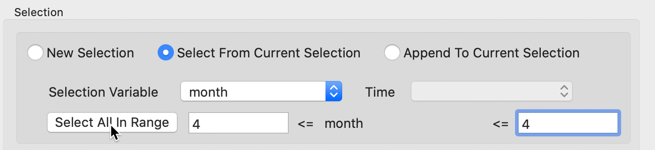
Figure 13: Select Month From Selection

Selecting the final list of variables

Our immediate objective is to save the selected observations as a new table. However, before we proceed with that, we want to remove some variables that we are really not interested in or that don’t contain useful information. For example, both month and year have the same value for all selected entries, which is not very meaningful. Also, a number of the other variables are descriptive strings, that do not lend themselves to a quantitative analysis. To reduce the number of variables contained in the data table, we will use the Table > Delete Variable(s) function (invoke from the menu or use right click in the table).

For our analysis, we will only keep Creation Date, Street Address, Zip Code, X Coordinate, Y Coordinate, Ward, Police District, Community Area, Latitude and Longitude as variables. All the other variables will be deleted. In the Delete Variables dialog, we select them and remove them from the table. The resulting set of variable headings should be as in Figure 14.

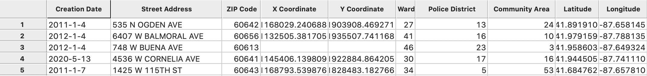
Figure 14: Data table with selected variables

Saving the data table

So far, all operations have been carried out in memory, and if we close GeoDa, all the changes will be lost. In order to make them permanent, we need to save the selected observations to a new file. While we initially read the data from a csv file, we will save the selected observations as a new table in the dbf format using File > Save Selected As. We next select dBase Database File from the available output formats and specify vehicles_April_2020.dbf as the file name.

However, there is a minor problem. The dbf file format is extremely picky about variable names (e.g., no more than 10 characters, no spaces) and several of the variable names from the Chicago Open Data Portal do not conform to this standard. GeoDa flags the violating variable names and suggests new field names, as shown in Figure 15.

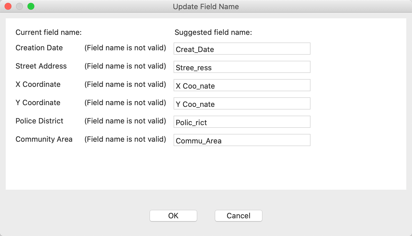
Figure 15: Variable Name Correction Suggestion

Since the suggested names are less than intuitive, we manually enter new variable names, as in Figure 16.

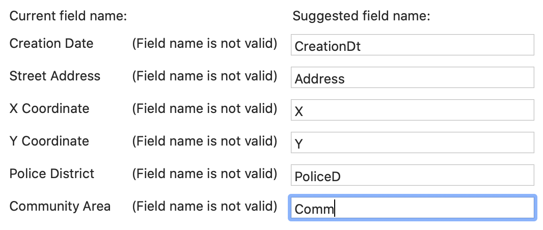
Figure 16: Variable Name Correction Suggestion

Now, we can safely save the file.

We close the current project by selecting File > Close from the menu, or by selecting the Close icon from the toolbar (the second icon from the left). Make sure to reply that you do not want to save any changes if prompted.

A final check

We check the contents of the new file by selecting the Open icon and dragging the file vehicles_April_2020.dbf into the Drop files here area. The table will open with the new content. The status bar reports that there are 1383 observations. The new variable names appear as the column headers, as shown in Figure 17.

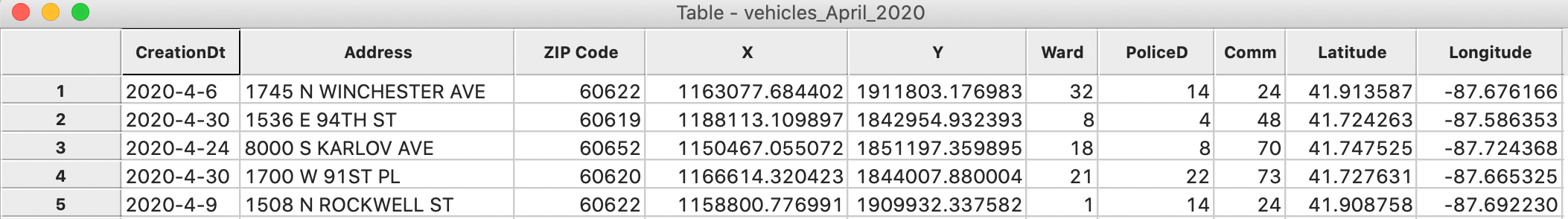
Figure 17: New vehicles data table

However, upon closer examination, there are some important missing values in the table. Sorting on either Latitude or Longitude will reveal 14 observations without these coordinates, as in Figure 18.

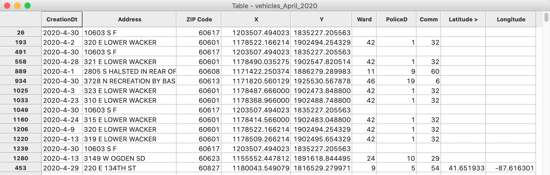
Figure 18: Missing lat-lon values

Similarly, sorting on either X or Y will show that 10 observations have no such coordinates, although they do have Latitude and Longitude, shown in Figure 19.

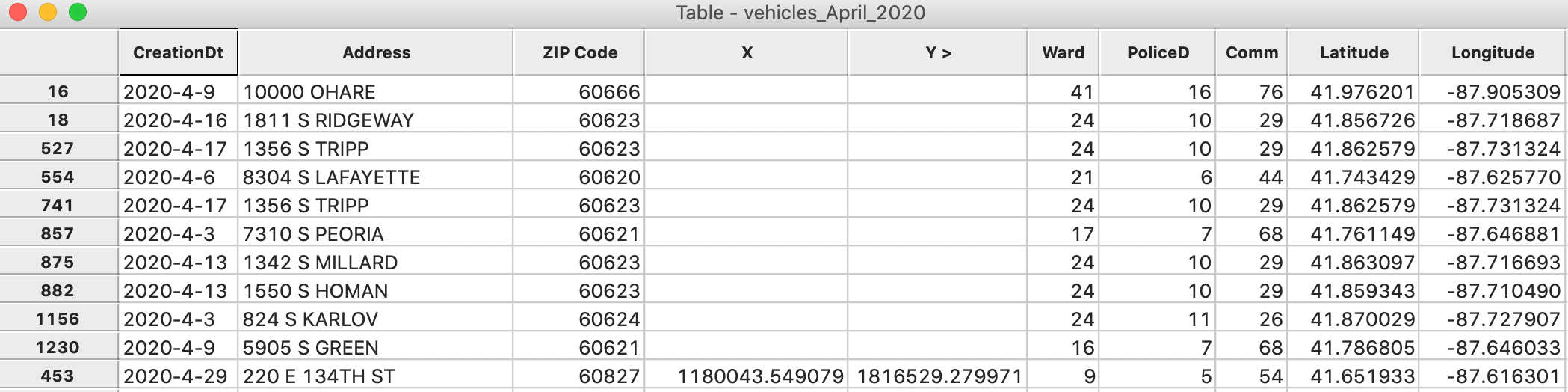
Figure 19: Missing x-y coordinates

More importantly, 7 observations have no code for Ward, PoliceD or Comm, as in Figure 20.

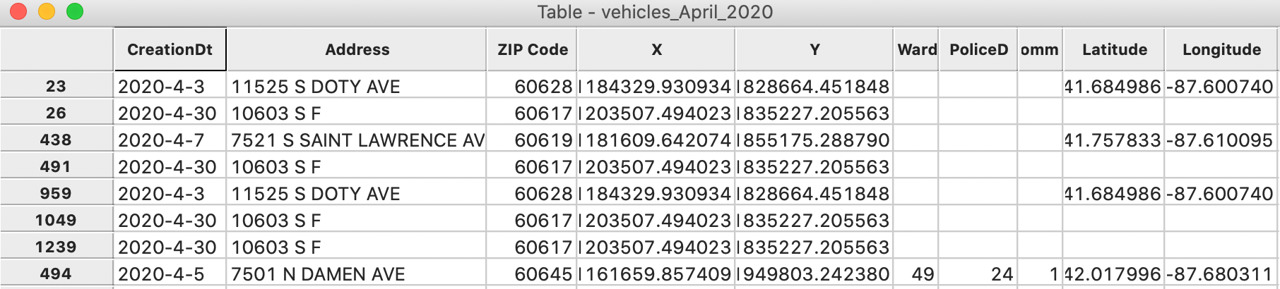
Figure 20: Missing codes for Community Area

For our analysis, we will either have to drop these observations, or, depending on the research question, find a way to impute some of the missing values. Given that our ultimate objective is to create a map for community areas, we want to make sure that as many observations as possible have a valid identifier for that area. As it happens, all the observations with missing Community Area codes do have valid x-y coordinates (even though some of them do not have valid lat-lon). Therefore, we will use the x-y coordinates to create a point layer. Also, there are fewer missing values for x-y than for lat-lon.

Inserting a unique identifier

In order to facilitate later operations that might involve merging different files, we want to make sure that each point is uniquely identified. As it stands, there is no such identifier in the current table.²

We add a new variable PTID as an integer and insert it before the first column (Table > Add Variable). We then use the left-most tab of the Calculator, labeled Special, and select the ENUMERATE operator, as in Figure 21.

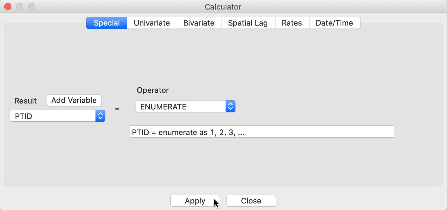
Figure 21: Create a unique identifier for the points

The variable PTID is added as a unique identifier for each observation, as in Figure 22. Note that the value of PTID depends on the order of the observations when it was created, so it may differ slightly if the order was not the original.

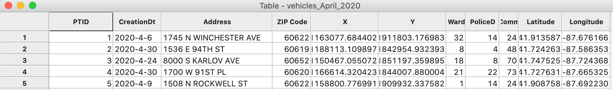
Figure 22: New vehicles data table

We can now save the new table to replace the current one (same file name), or use Save As to specify a new file name. To keep the files distinct, we use the latter option and create a new file as vehicles_April_2020_id.dbf.

Creating a Point Layer

So far, we have only dealt with a regular table, without taking advantage of any spatial features. However, our table contains fields with coordinates. Therefore, GeoDa can turn the table into an explicit spatial points layer that can be saved in a range of GIS formats. We can then use the spatial join functionality to determine the community area for those locations (points) that have missing values.

Creating a point layer from coordinates in a table

In GeoDa, it is straightforward to create a GIS point layer from tabular data that contain coordinate information. The process is started from the main menu, as Tools > Shape > Points from Table, or by selecting the same item from the Tools toolbar icon. After invoking the function, a dialog appears to let you specify the X and Y coordinates.

In our example, the table contains two sets of coordinates, X and Y, as well as Longitude (the horizontal, or x-coordinate) and Latitude (the vertical, or y-coordinate). Given that the observations with missing community area codes all have X-Y coordinates, we will employ the latter to create a point layer.

Projection information

It is easy to create a point layer with just the coordinates, but without any projection information. However, as a result, there will be no such information associated with the layer, which is problematic for future spatial manipulations. For example, the lack of a prj file (with projection information for a shape file) will create problems when we want to use the multi-layer feature in GeoDa to find out in what community area the points are located. For this to work properly, both layers need to be in the same projection.

For Lat-Lon, this is not much of a problem, since those coordinates are not projected, which can be specified in a relatively straightforward manner. The CRS (coordinate reference system) that is used to refer to such layers is EPSG:4326, with associated proj4 definition:³

+proj=longlat +ellps=WGS84 +datum=WGS84 +no_defs

This is the information that needs to be entered in the CRS (proj4 format) box in the Save As dialog.

For the X-Y coordinates, this is much more of a challenge. It is usually extremely difficult (to impossible) to deduce the projection from the values for the coordinates, without further information. In our case, the City of Chicago open data portal does not contain any such metadata. So, basically, we would be stuck, were it not that we happen to know that the city traditionally has used the Illinois State Plane (feet) projection system for its data. This turns out to work, and we can enter the CRS information for EPSG:3435:

+proj=tmerc +lat_0=36.66666666666666 +lon_0=-88.33333333333333 +k=0.9999749999999999 +x_0=300000.0000000001 +y_0=0 +ellps=GRS80 +datum=NAD83 +to_meter=0.3048006096012192 +no_defs

The CRS information will allow us to create a point layer with the appropriate projection information. Note that GeoDa requires the complete CRS information, not just the EPSG code.

Point layer using X-Y

We create a point layer using X and Y as the coordinates. After invoking Tools > Shape > Points from Table, we select X and Y from the dialog, as shown in Figure 23.

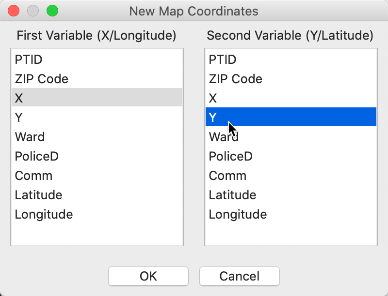
Figure 23: Specifying X-Y point coordinates

Once OK is pressed, the point map shown in Figure 24 appears on the screen. Note that only 1373 points are shown, since 10 out of the 1383 original observations do not contain a value for x-y. This is confirmed by the warning shown in Figure 25, which lists the row numbers of the observations with missing coordinates. While these points are not included on the map, they are still part of the data table.

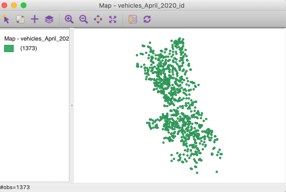
Figure 24: Point map for x-y coordinates

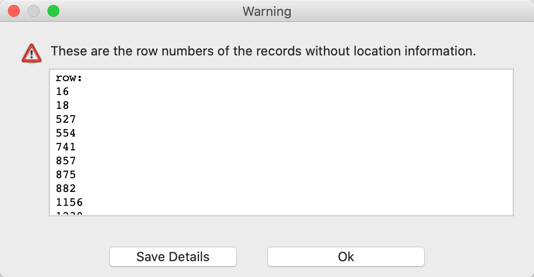
Figure 25: Observations with missing coordinates

To create a file with the geographic information, we select File > Save As and specify ESRI Shapefile (*.shp) as the file type in the dialog. Next we spell out a file name, such as vehiclepts_xy for the shape file. The full File Path will appear in the dialog. The final step is to provide a definition for the CRS in the proper proj4 format. We saw above what the entry should be for EPSG:3435 (Illinois State Plane Coordinates). With that entry in the CRS box, we can save the new file with the proper projection information.

Point layer cleanup

After completing the save operation, we close the current project (make sure to respond No to the query about saving the geography information). We next load the file vehiclepts_xy.shp. We get the same base map as in Figure 24, but we also continue to receive the warning. What happened?

Whereas the point map in Figure 24 only depicts the observations with valid coordinates, the file saved created a new table for all the data, including those observations without coordinate information. In order to create a clean point file where all the observations have valid x and y, we proceed as follows.

We select all the observations in the map window (make sure the number of selected = 1373), as in Figure 26.

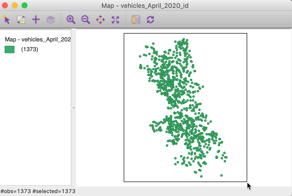
Figure 26: Selected points in x-y map

Next, instead of using Save As, we invoke Save Selected As, which will create a point layer that contains only the valid (selected) observations. We specify the file name as vehiclepts_xyc. Since the correct CRS is already contained in the dialog, we can click OK.

After closing the project and loading the new file, the resulting base map is shown without the warning.

Community Area Boundary File

Extracting the community area layer

We resort to the City of Chicago open data portal again to obtain the boundary file for the Community Areas. From the opening screen, select the button for Facilities & Geo Boundaries. This yields a list of different boundary files for a range of geographic areal units, as shown in Figure 27.

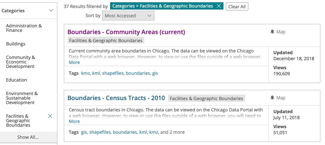
Figure 27: Chicago data portal Boundary Files

We select Boundaries - Community Areas (current), which brings up an overview map of the geography of the community areas of Chicago, as in Figure 28.

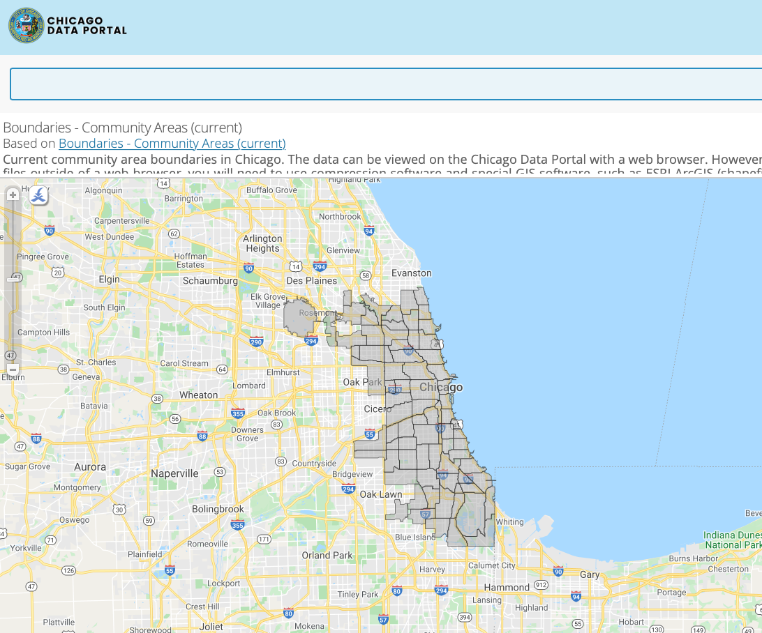
Figure 28: Chicago Community Areas geographic boundaries

When we choose the blue Export button in the upper right hand side of the web page, a drop down list is produced with the different export formats supported by the site. As illustrated in Figure 29, we select Shapefile, the ESRI standard for boundary files.

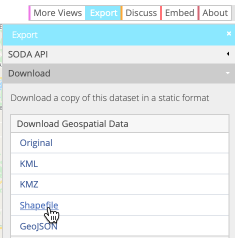
Figure 29: Download boundaries as a shape file

This will download a zipped file to your drive that contains the four basic files associated with a shape file, with file extensions shp, shx, dbf and prj. The file name is the rather uninformative geo_export_9af88a41-660e-4b6a-91e3-b959e3e51ced (it may differ slightly for downloads carried out on different dates).

Community Areas base map

To generate a base map for the community areas, we start a new project in GeoDa and drop the just downloaded file into the Drop files here area of the data source dialog. This will open a green base map, as shown in Figure 30. Note how the status bar lists the number of observations as 77.

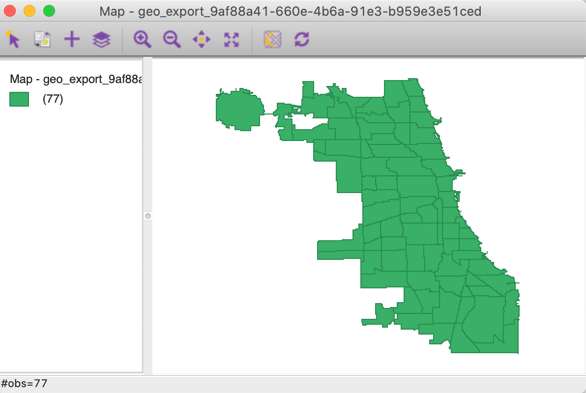
Figure 30: Community Area Base Map

We will return to the mapping functionality later. First, we check the contents of the data table by clicking on the Table icon in the toolbar. The familiar table appears, listing the variable names as the column headers and the contents for the first few observations, as in Figure 31.

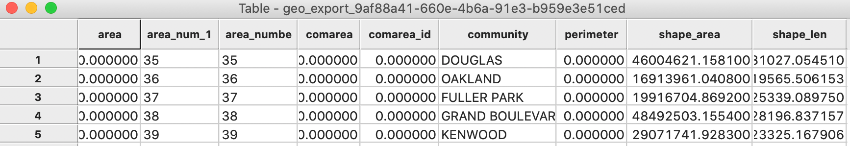
Figure 31: Community Areas initial data table

When we examine the contents closer, we see that we may have a problem. The values for area_numbe and area_num_1 (which are identical), corresponding to the Community Area identifier, are aligned to the left, suggesting they are string variables. For effective use in selecting and linking observations, they should be numeric, preferably integer.

We again use the Table > Edit Variable Properties functionality to change the variable format. We proceed as before, but now change the string format to integer. After the conversion, we will see the values for area_num_1 right aligned in the table, shown in Figure 32, as numeric values should be.

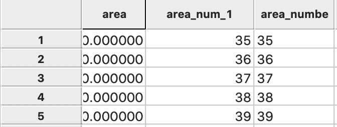
Figure 32: Community ID as Integer

Finally, we do some cleanup and delete all the variables we will not need. We end up with just two variables: area_num_1 (the community area ID) and community (the community are name).

Changing the projection

There is one more wrinkle. The downloaded layer is expressed as lat-lon coordinates and thus is unprojected. We can verify this by selecting Save As and checking the contents of the CRS box, which is as in Figure 33.

Figure 33: CRS entry for lat-lon (unprojected)

However, the point layer we just created is in Illinois State Plane coordinates. In order for the two layers to be compatible, we need to reproject the current base map. There are two ways through which we can accomplish this. Both use Save As, in which we first specify a new file name, say commarea. Next, we need to enter the correct information in the CRS box. We can manually enter the proper definition for CRS:3435, as we did for the point layer. Alternatively, we can click on the small globe icon to the right of the CRS specification. This brings up a Load CRS from Data Source dialog. We now can drop the file vehiclepts_xy.shp into the Drop files here area and the CRS expression will be updated to the one from that point file, as in Figure 34.

Figure 34: Partial CRS entry for Illinois State Plane projection

Selecting OK will save the file in the correct projection.

To verify the reprojection, we close the project and load the file commarea.shp. The base map is now as in Figure 35. Compared to Figure 30, the new base map has a slightly different orientation and the spatial units are somewhat compressed relative to the unprojected version.

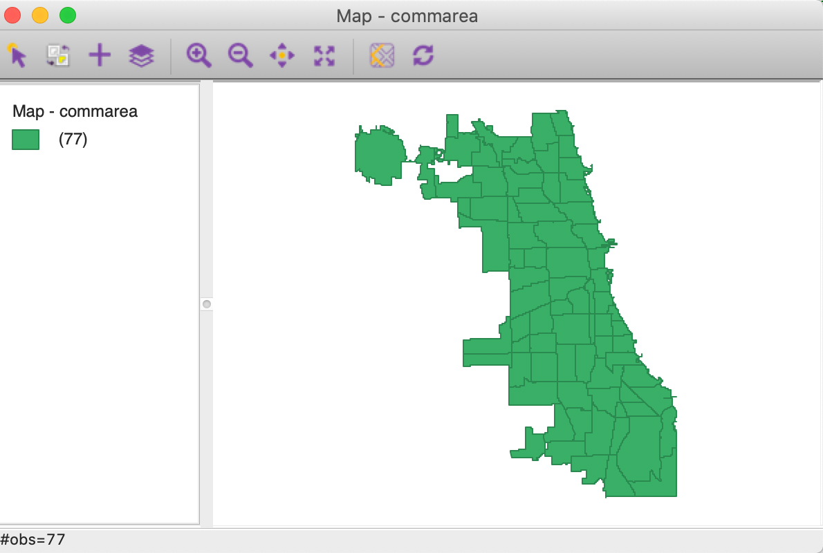
Figure 35: Community Area Base Map

Abandoned Vehicles by Community Area

Our ultimate goal is to map the abandoned vehicles by community area. But, so far, what we have are the individual locations of the vehicles. What we need is a count of the number of such vehicles by community area. In GIS-speak, this is referred to as spatial aggregation or spatial join. The simplest case is the one we will illustrate here, where all we need is a count of the number of observations that fall within a given community area.

We will approach this in two different ways. In the first, we will simply carry out the spatial join to add the number of vehicles as an additional field to the data table of commarea. However, we have a small problem, in that the point layer for the vehicles is short of 10 observations. Therefore, we also tackle the problem in a slightly more circuitous way. We first use a different form of spatial join to obtain an areal identifier (the community area) for each point. Because all the points with missing community areas have x-y coordinates, we can use the vehiclepts_xyc file for that, even though it is missing 10 points. We then use the merge functionality to add the missing community areas to the original vehicle file and employ aggregate to compute the total points in each area.

Spatial join – count points in area

The spatial join is part of the limited multilayer functionality that has been implemented in GeoDa. In order to fully understand how this works, it is important to keep in mind that whatever is to be computed can only be added to the first layer, which is the layer loaded when opening a project. In our example, since we want to add a count of vehicles by community area to the community area layer, the first file is commarea. We add a second layer by means of the plus (+) icon in the base map window. This is the point layer, vehiclepts_xyc (containing only points with valid x-y coordinates).

The resulting map window is as in Figure 36.⁴ The Map Layer Settings dialog shows the commarea layer on top of the vehiclepts_xyc layer.

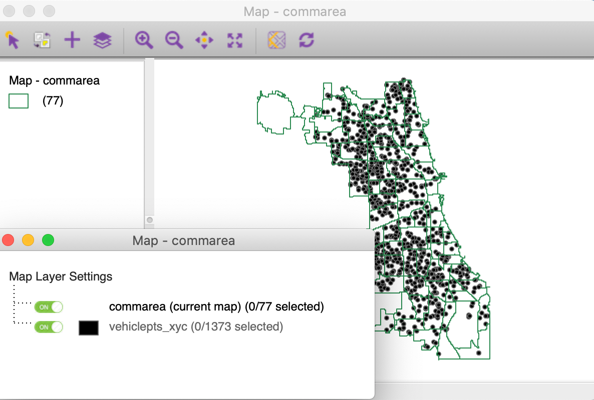
Figure 36: Multiple layers - option 1

We start the counting procedure by invoking Tools > Spatial Join. The Spatial Join dialog in Figure 37 specifies the current map, i.e., the layer to which the information will be added. As mentioned, this is always the first layer loaded. In our example, this is commarea. Next is a drop down list with all possible layers that can be joined. In our case, there is just one, vehiclepts_xyc. The default is a Spatial Count, i.e., a simple sum of the number of observations from the points layer that fall inside each community area. It is also possible to calculate more complex joins, such as the sum or median of observations, but that is beyond the current scope. Since we don’t use an actual variable in the spatial count, the Join Variable and Join Operation entries remain blank.

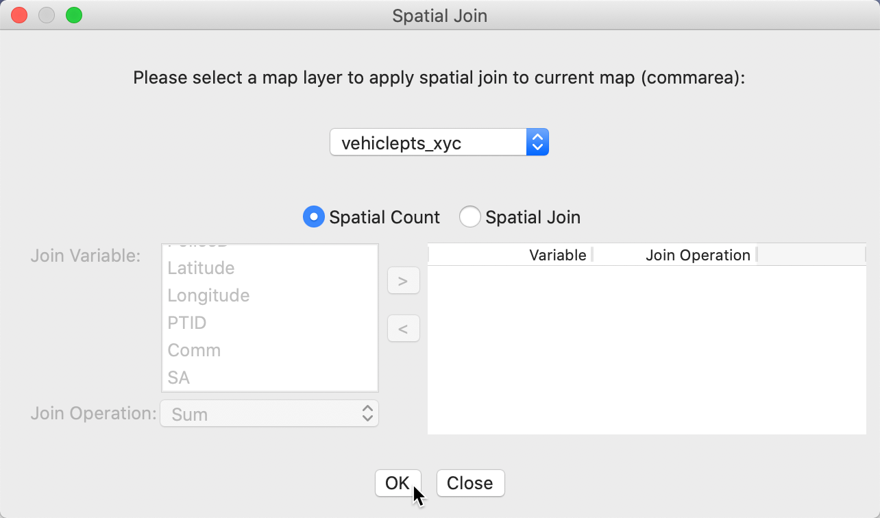
Figure 37: Spatial count dialog

Clicking OK brings up a variable name selection dialog. We stay with the default SC and complete the calculation. The result is a new column of vehicle counts added to the data table. Save the table to make this computation permanent.

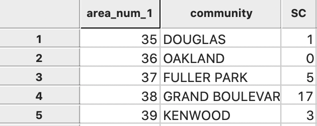
Figure 38: Spatial counts added to community area layer

If the points layer were complete, this is all we would have to do. However, we will try to get a full count of all the vehicles, not just the ones with valid x-y. This is carried out next.

Spatial join – area id for each point

We now load the files in the reverse order, with the vehiclepts_xyc layer first and the commarea layer added through the + icon. The resulting base map is as in Figure 39.

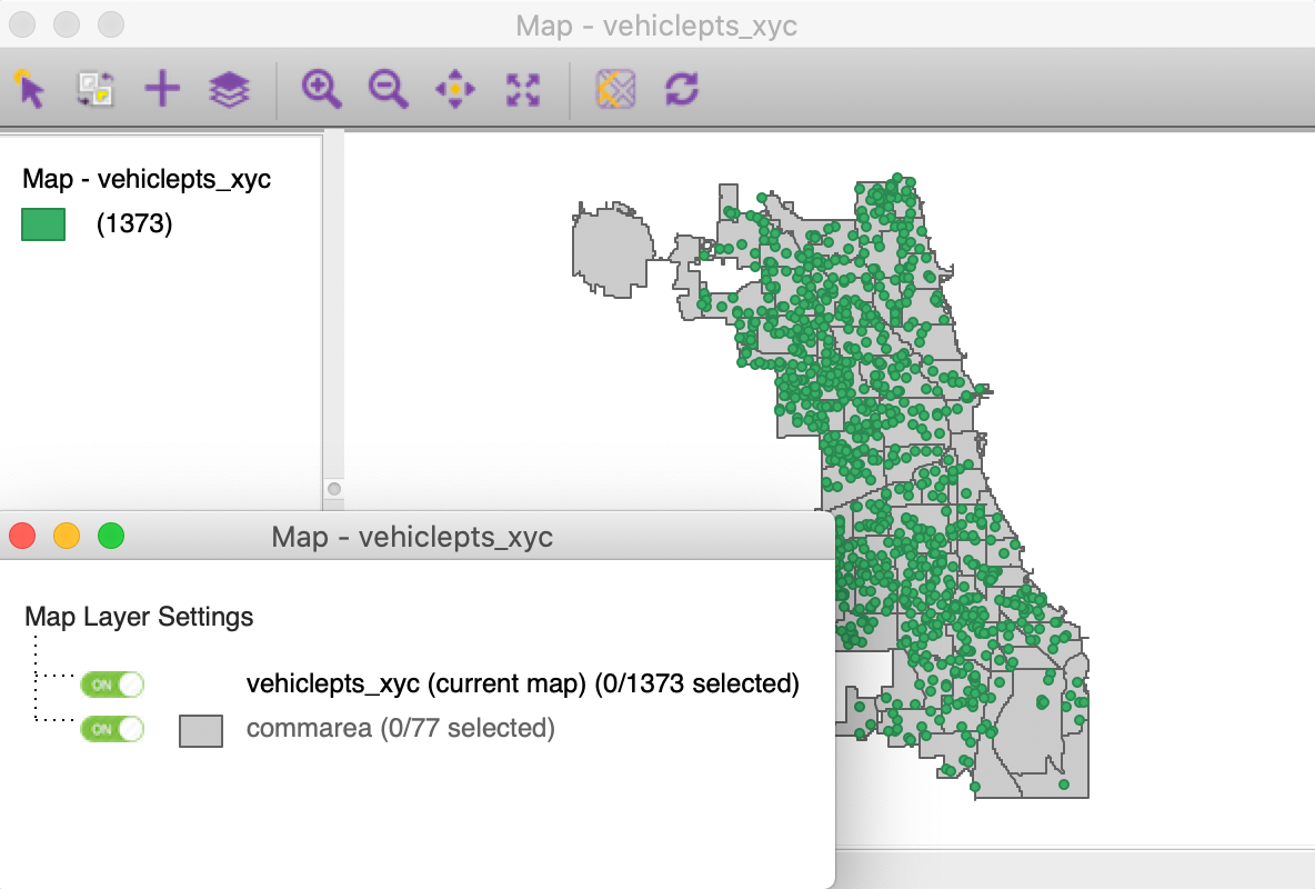
Figure 39: Multiple layers - option 2

We invoke Tools > Spatial Join. This time, the Spatial Join dialog is slightly different, as in Figure 40. The current map is vehiclepts_xyc and the drop down list for the other map layers gives commarea as the (only) entry. In order to make sure that the community area identifier is added to the point layer, we set ID Variable to area_num_1. We click OK to select the variable name and keep the default SA.

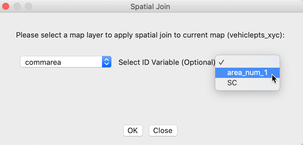
Figure 40: Spatial join dialog

The result is a field for SA added to the data table of the vehicle points. In Figure 41, the point identifier PTID, Comm and SA are shown next to each other, after sorting on Comm. The missing codes correspond to community areas 51, 52 and 69 (the order of observations may differ slightly). We Save to make the table permanent.

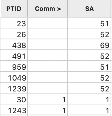
Figure 41: Community ID added to vehicle point layer

Merging the new identifiers into the original point data set

The new data set for vehiclepts_xyc has a full set of community area identifiers, but for an incomplete set of points. On the other hand, the original point data set vehicles_April_2020_id has all the points, but not all the identifiers.

We will merge vehiclepts_xyc.dbf with vehicles_April_2020_id.dbf and then manually complete the community identifiers by editing the table. We load the latter file first and next select Table > Merge. This brings up the Merge dialog, as shown in Figure 42. We set the key values to PTID in both tables and only bring in the new variable SA. Merge adds the new column to the vehicles_April_2020_id table.

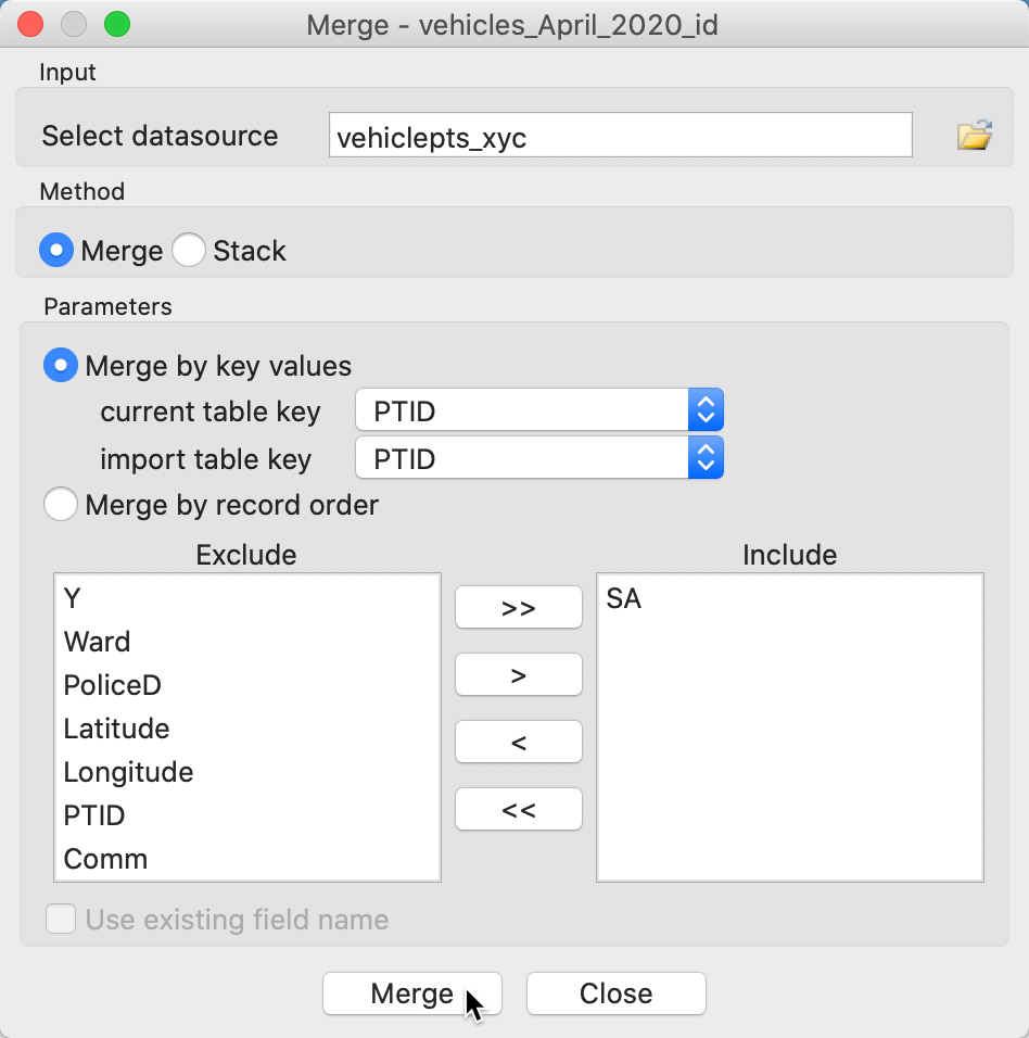
Figure 42: Merge dialog

The next step is very manual. We sort on the Comm variable and manually edit each of the empty cells by clicking on them and entering the value from the matching SA entry, as in Figure 43. We complete the process by saving the edited table. Alternatively, we could have sorted on SA and enter the missing values from Comm. It does not matter which field is used, as long as one of them has entries for every observation.

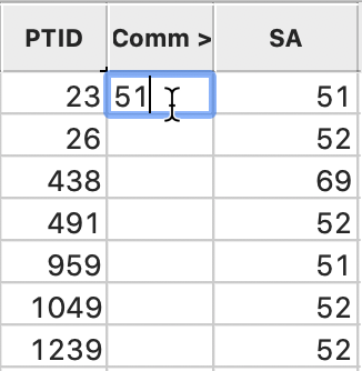
Figure 43: Editing the merged community ID fields

A word of caution

Upon closer examination of the values for the community indicator SA, we find several values of -1. Clearly, this is not a valid community area indicator, but it means that the coordinates of the point in question could not be located inside any of the boundaries of the community areas. Why would this be the case?

So far, we have taken the downloaded information at face value, but there may be imprecisions in the recorded coordinates. Similarly, the boundary values for the community areas may show slight mismatches with the points, typically close to the border of an area. As a result, it is quite likely that whenever different spatial data sources are combined (i.e., the point coordinates from one file and the area boundaries from a different source) spatial mismatches may result. How we address these depends on the context. For the sake of simplicity, we have chosen to just use the encoded community areas and provide the missing values from our point in polygon exercise. We could also have gone the other route and added the information from the comm variable to the locations with missing x-y coordinates and those with a mismatch from the SA variable. Even more radically, we could have geo-coded the points with missing coordinates from the original address information.

This illustrates the many often ad hoc choices one needs to make in an actual data wrangling process.

Aggregation

Since every point in the vehicles_April_2020_id table now has a community area value in the comm field, we can use this value to aggregate the points by community area. This is an alternative way to obtain the count of vehicles in each area. We invoke the Table > Aggregate command and select Comm as the key in the dialog, shown in Figure 44.

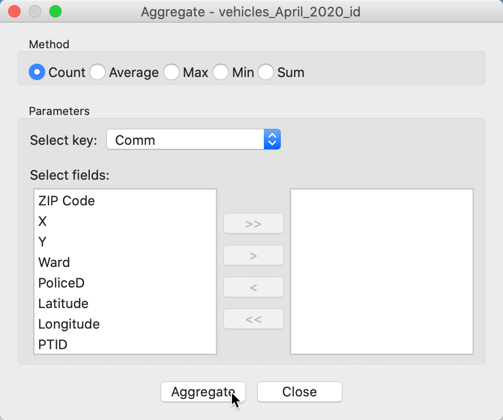
Figure 44: Aggregate dialog

We need to specify a file name for the output, say veh_count.dbf. After the aggregation process is completed, the new file contains two fields, one for Comm, and the other for the number of vehicles in the area, AGG_COUNT, as in Figure 45.

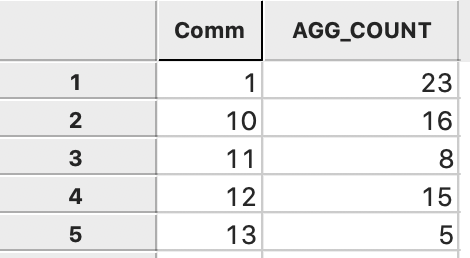
Figure 45: Aggregated count by community area

At this point, we move back to the commarea file (close the project and load the shape file) and use Table > Merge to merge the vehicle counts into the community area layer. In the Merge dialog, we specify area_num_1 as the key in the area layer and Comm as the key in the import file, As in Figure 46. We only include the variable AGG_COUNT.

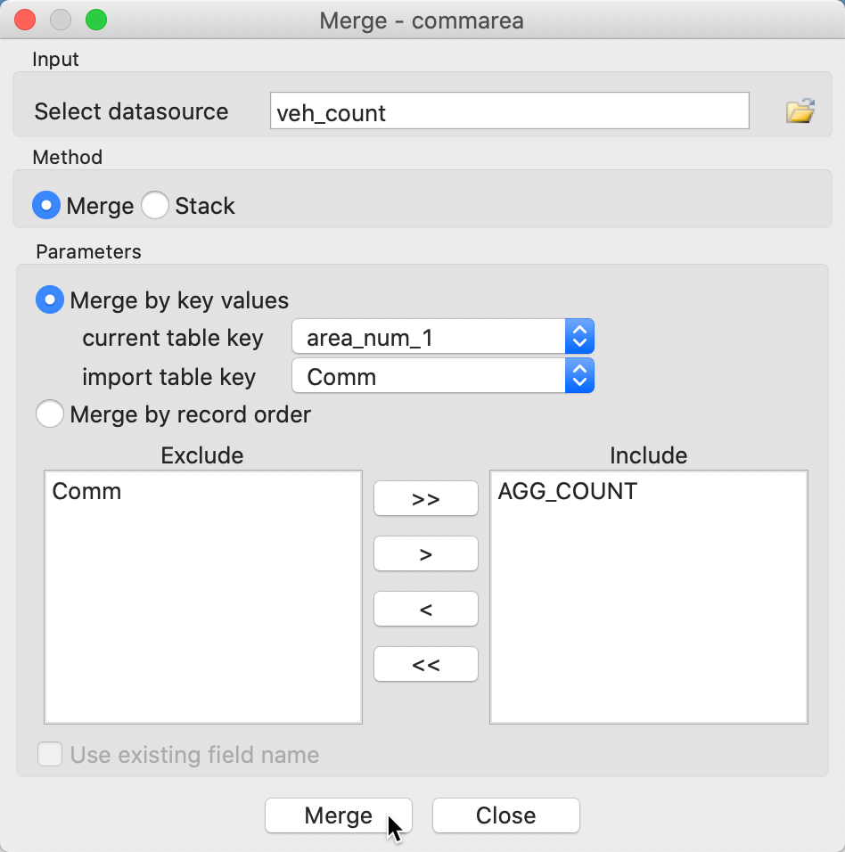
Figure 46: Merge counts into community areas

This results in the new field to be added to the area layer, as in Figure 47. Note how area 36, Oakland, has a value of 0 with the first approach, but an empty value for the second approach. The missing value is the result of the absence of the id 36 in the Comm fields of the point data set. As a result, no aggregation is carried out and there is no entry for that area. In contrast in the other spatial join, the number of points within each area is counted, which results in 0 for area 36.

Upon closer examination of the SC and AGG_COUNT fields, we find a number of subtle differences between them. These have several causes. First of all, there were points with missing x-y coordinates, and thus they were not contained in SC. In addition, there are a number of small spatial mismatches, especially when points are very close to the boundary of a community area. However, in the end, these minor differences will not matter for our map, since the counts need to be divided by the (much larger) population total to yield per capita results. We next turn to obtaining the population data.

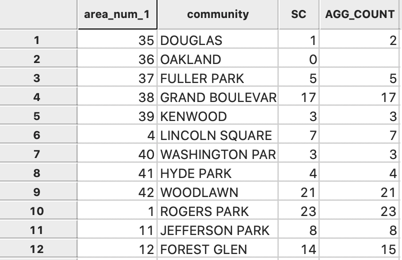
Figure 47: Aggregated count added to community area layer

Community Area Population Data

So far, we only have information on the abandoned vehicles. As it turns out, obtaining data for the population by community area is not that straightforward. The City of Chicago web site contains a pdf file with the neighborhood ID, the neighborhood name, the populations for 2010 and 2000, the difference between the two years and the percentage difference. While pdf files are fine for reporting results, they are not ideal to input into any data analysis software. Since there are only 77 community areas, we could sit down and just type the values, but that is asking for trouble. Instead, we could use a web scraping tool and special software to extract the information from a pdf file, but that would be quite burdensome.

Some more sleuthing reveals that the Chicago Metropolitan Agency for Planning (CMAP) has a Community Data Snapshots site that contains a host of census data for the Chicago region, including population by community area for 2000 and 2010. As seen in Figure 48, there is a csv table with Chicago Community Area data, as well as a pdf file with detailed descriptions of the fields.

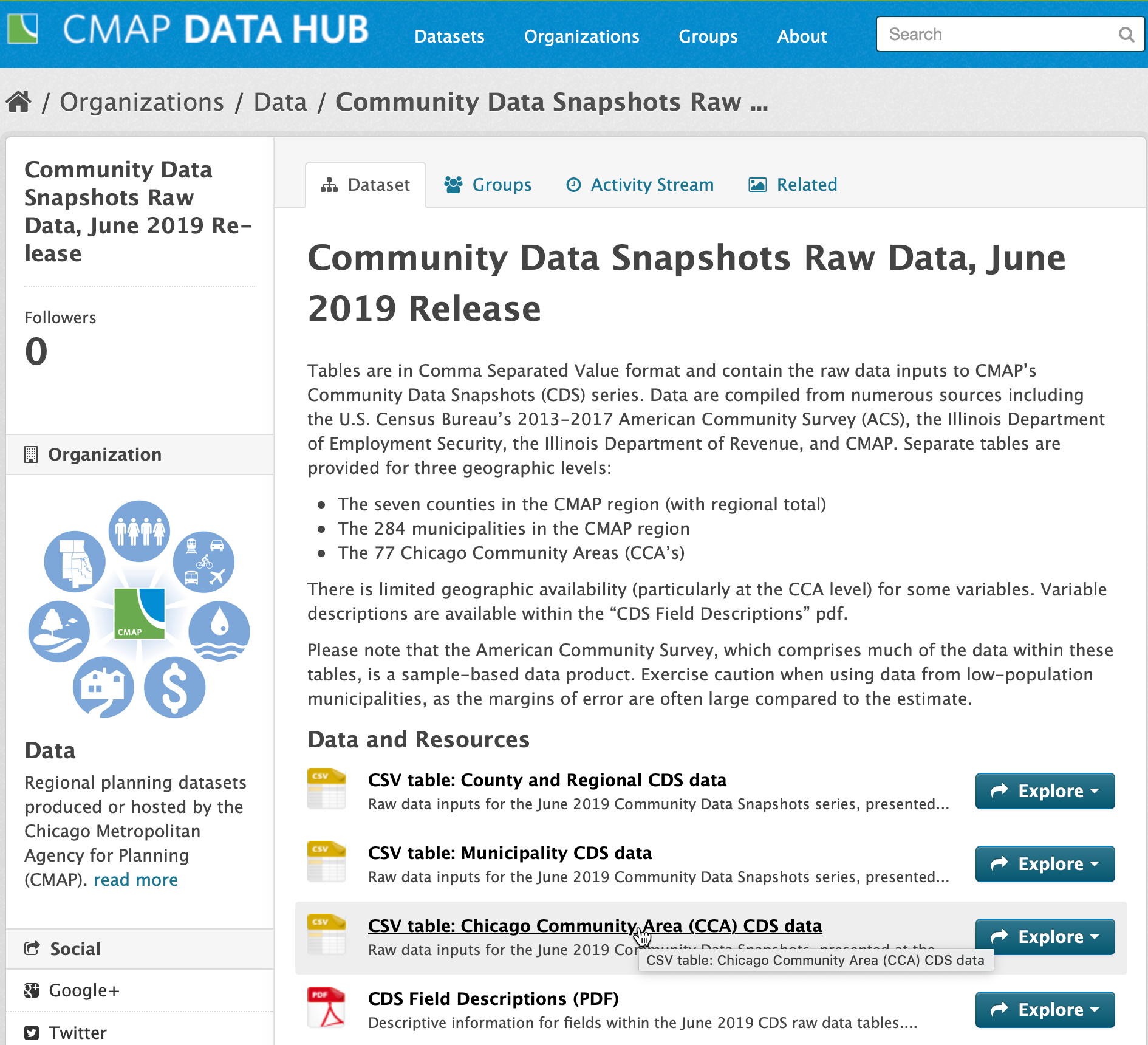
Figure 48: CMAP community data snapshots

Community area population data table

After we download the csv file, we can load it into GeoDa. The associated data table is shown in Figure 49. In addition to the population figures, the table contains many other variables that we don’t need. We use Table > Delete Variable(s) to remove everything except the community identifier and the two population totals.

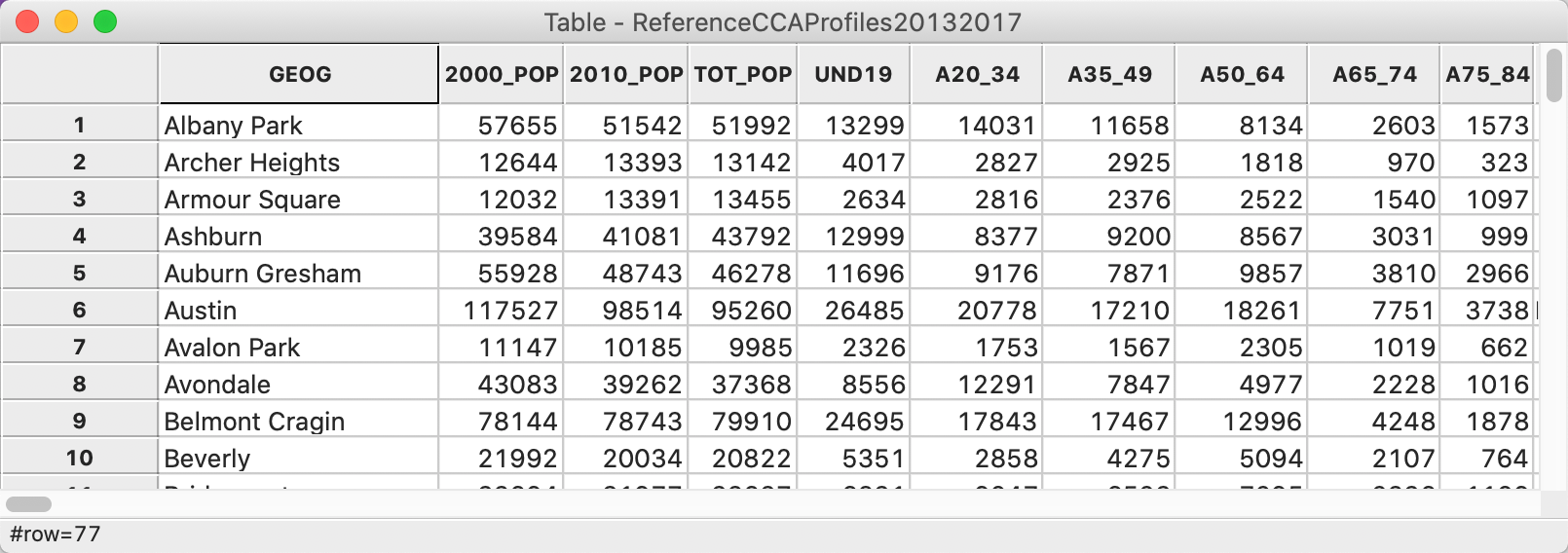
Figure 49: CMAP community data table

However, there is another problem. The table lacks the usual unique identifier for the community areas, which are listed alphabetically by name. In order to implement a merge operation, we need an integer identifier for each observation. We create a new variable as alpha_id and use the calculator Special tab with the ENUMERATE operator to add a simple sequence number to the table (similar to what we did with the points data set). The resulting table is as in Figure 50. We use Save As to create a new dbf file with the population data, cmap.dbf.

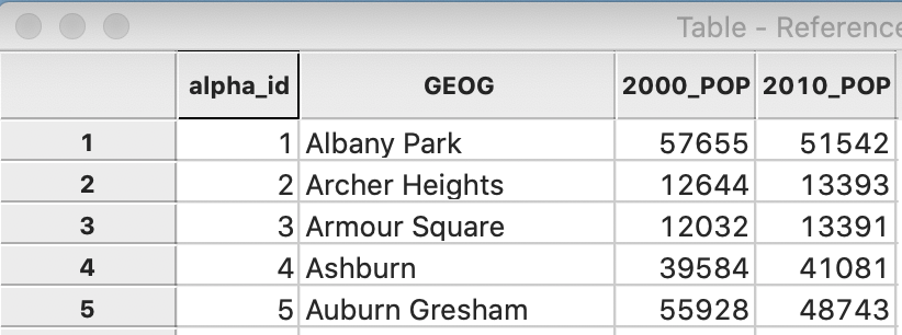
Figure 50: CMAP community data table with identifier

Merging the population data into the community area layer

The next step is to merge the new cmap.dbf file into the community area layer. In order to implement that, we need a matching unique identifier in each table, but we currently don’t have such an identifier. We could simply add a sequence number to the commarea table, after sorting the observations alphabetically by community area name, but there is a catch. In the CMAP data set, the loop area is referred to as THE LOOP, whereas in the date from the city data portal, it is called LOOP (without THE). As a result, the sequence numbers for the alphabetical order in the two tables will not match.

For this to work, we need to first edit the name for the loop area to be consistent between the two tables. We do this in the commarea table by clicking on the proper cell and inserting the edit, as in Figure 51. Now, the name for this area is THE LOOP in both tables.

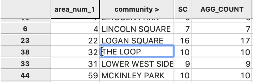
Figure 51: Editing the loop identifier

A final step before the merge operation is to sort the table alphabetically by the (new) community area names (click on the field name and make sure the sorting order is >) and adding a sequence number in the same way as before. The table will now be as in Figure 52. We save the table to make the changes permanent.

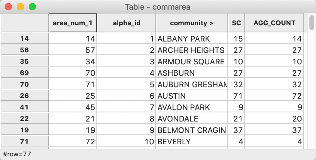
Figure 52: Community area layer with alphabetic order identifier

We are now ready to merge the cmap.dbf file into the community area layer. We specify alpha_id as the common key in both tables, as in Figure 53. In addition to the two population variables, we also include the area name (GEOG) to allow for a final consistency check. It is generally good practice to initially include both keys in the merged data set to make sure that they match.

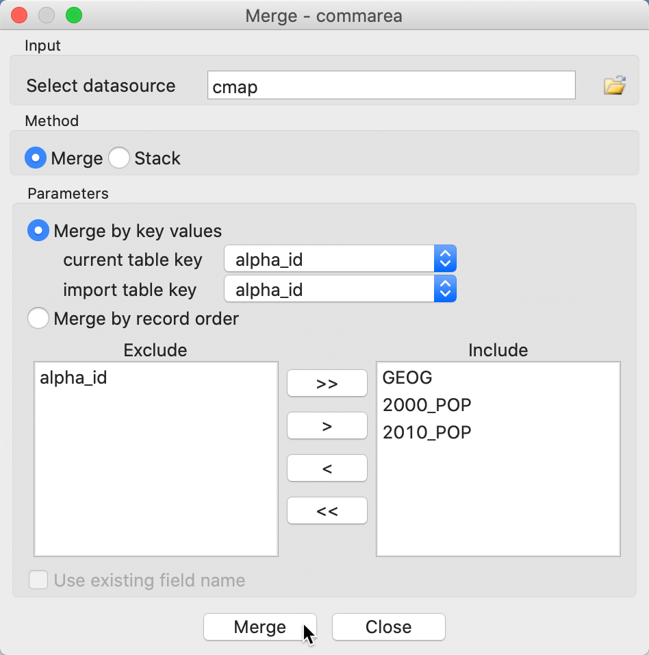
Figure 53: Merging the cmap data into the community area layer

The resulting merged table, shown in Figure 54, now contains all the information we need to compute and map the abandoned vehicles per capita. We again save the table to make the changes permanent.

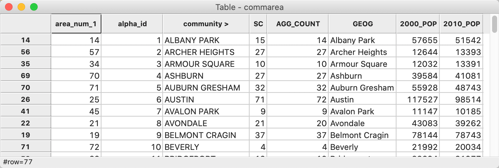
Figure 54: Community area layer with population data

Mapping Community Area Abandoned Vehicles Per Capita

Variables that represent counts, like the number of abandoned vehicles or the area population are so-called spatially-extensive variables. Everything else being the same, we would expect there to be more abandoned vehicles where there are more cars (people). Consequently, mapping spatially extensive variables may not be that informative. In fact, it may actually be quite misleading since such variables are basically correlated with size.

In order to correct for that, maps should represent spatially-intensive variables, such as rates and densities. To make our final map, we therefore have to first compute the per capita rate.

Abandoned vehicles per capita

We first use Table > Add Variable to create a new (real) variable, say vehpcap. Next, we use the Bivariate tab in the Calculator with the DIVIDE operator to divide SC by 2010_POP. In order to make the result a bit more meaningful, we turn it into abandoned vehicles per 1000 people. Therefore, we use the MULTIPLY operator to multiply vehpcap by 1000. The result is as in Figure 55. We save the table to make it permanent.

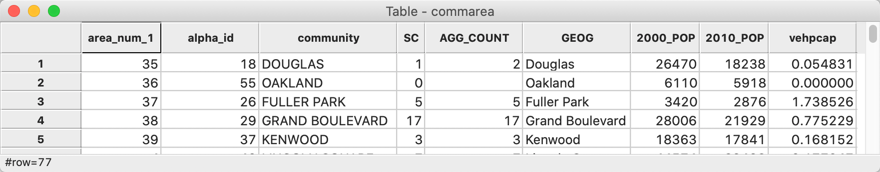
Figure 55: Abandoned vehicles per capita

Quantile map

We create a simple quintile map with the observations ordered into five quantiles. We select the map icon in the toolbar and choose Quantile Map with 5 categories, as in Figure 56.

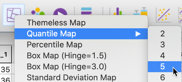
Figure 56: Quantile map command

With vehpcap as the variable and clicking on the OK button, the quintile map appears as in Figure 57. Because 77 (the number of observations) does not divide cleanly into 5, three categories have 15 observations and two have 16 (in a perfect quintile world, they each should have exactly the same number of observations). The number of observations is given within parentheses in the legend. The intervals for each of the 5 categories are given in the legend as well.

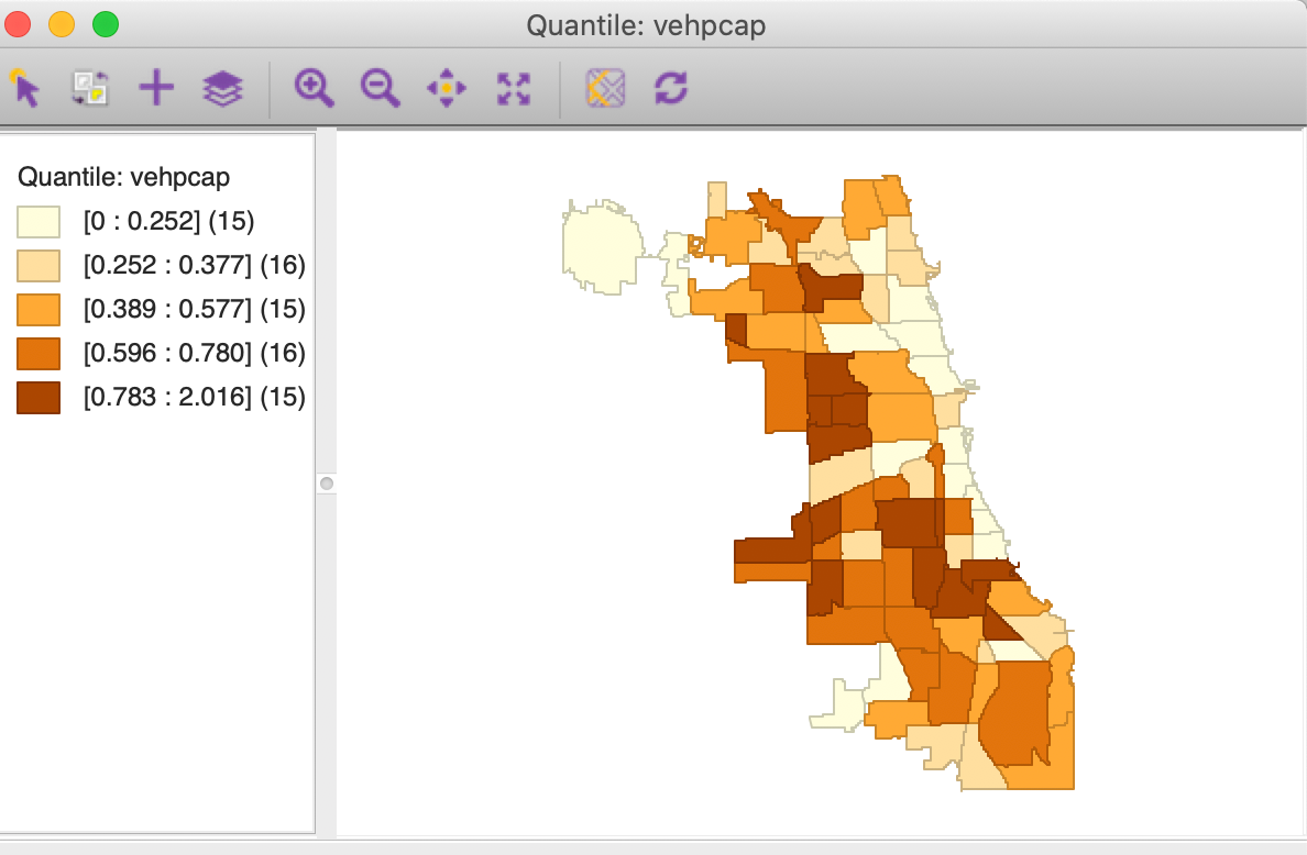
Figure 57: Quantile map for abandoned vehicles per capita

This ends our journey from the open data portal all the way to a visual representation of the spatial distribution of abandoned vehicles. The map does suggest some patterning and some potential association with proximity to the major interstates. Also, we may be interested in the degree to which the spatial pattern for April 2020 is similar to that for other years, or for other months. We leave a more formal analysis of patterns (and clusters) to later chapters.

The moral of the story is that careful attention needs to be paid at every step of the way. Even though lots of information is provided through open data portals, metadata are often missing, and there are many quality issues as well as inconsistencies in the way the data are recorded. Data wrangling is still very labor intensive. Although much progress has been made in terms of automated tools (for big data), in practice, there remain many edge cases and gotcha situations. User beware!

GeoDa

An Introduction to Spatial Data Science

Spatial Data Wrangling (3) – Practice

Luc Anselin1

09/16/2020 (updated)