Contiguity-Based Spatial Weights

Introduction

In this chapter, we will begin to explore the spatial weights functionality in GeoDa. We focus initially on spatial weights based on the notion of contiguity between polygons. We will use the ncovr sample data set with socio-economic data related to homicides in U.S. counties set that comes pre-installed with GeoDa.

After a brief review of important concepts, we consider rook and queen contiguity-based weights, as well as higher order contiguity. We highlight the importance of the Project File to keep track of weights metadata. We next examine the characteristics of the weights using the connectivity histogram, and explore the connectivity map and connectivity graph. The connectivity information can also be exploited to select locations with their neighbors.

Distance-based weights and some more advanced concepts are covered in the chapters that follow.

Objectives

• Construct rook and queen contiguity-based spatial weights

• Compute higher order contiguity weights

• Store the weights information in a GeoDa Project File

• Assess the characteristics of spatial weights

• Visualize the graph structure of spatial weights

• Identify the neighbors of selected observations

GeoDa functions covered

• Weights Manager (Tools > Weights Manager)
  • weights file creation interface
  • ID variable
  • rook and queen contiguity
  • precision threshold option
  • spatial weights file name
  • weights properties in the weights manager
  • loading weights from a file
• Structure of a GAL file
• File > Save Project
• Connectivity histogram
• Connectivity map
• Connectivity graph
• Select neighbors of selected
  • Map > Connectivity
  • Table > Add Neighbors To Selection

Preliminaries

We again use a data set that is comes built-in with GeoDa and is also contained in the GeoDa Center data set collection.

• ncovr: homicide and socio-economic data for 3085 U.S. counties

You can either load this data from the Sample Data tab, or, if you previously downloaded the files, drop the natregimes shape file into the usual Drop files here box in the dialog. This yields a themeless base map of the U.S. counties, shown in Figure 1.

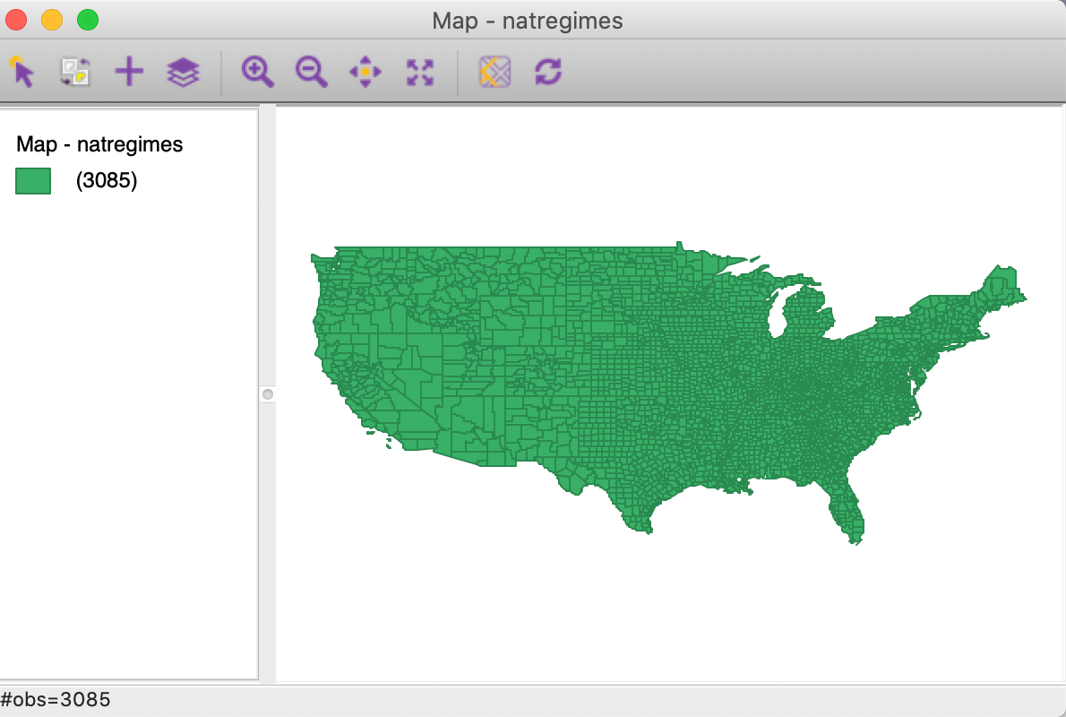
Figure 1: U.S. counties themeless map

If you used the file from the Sample Data collection in GeoDa, a copy of this data should be created to make sure that the weights files we are about to construct end up in the same directory as the data. To this effect, invoke File > Save As to create a duplicate of the respective files in a working directory (choose ESRI Shapefile as the file type).

Close the project and load the new file in the usual fashion. In the example that follows, the file name is natregimes (with four matching files with extensions .shp, .shx, .dbf, and .prj).

If you loaded natregimes from a downloaded folder, you do not need to carry out this extra step.

We are now ready to proceed.

Spatial Weights - Basic Concepts

Spatial weights are a key component in any cross-sectional analysis of spatial dependence. They are an essential element in the construction of spatial autocorrelation statistics, and provide the means to create spatially explicit variables, such as spatially lagged variables and spatially smoothed rates.

Formally, the weights express the neighbor structure between the observations as a \(n \times n\) matrix \(\mathbf{W}\) in which the elements \(w_{ij}\) of the matrix are the spatial weights: \[\begin{equation*} \mathbf{W}=\left[ \begin{matrix} w_{11} & w_{12} & \ldots & w_{1n}\\ w_{21} & w_{22} & \ldots & w_{2n}\\ \vdots & \vdots & \ddots & \vdots\\ w_{n1} & w_{n2} & \ldots & w_{nn} \end{matrix} \right]. \end{equation*}\] The spatial weights \(w_{ij}\) are non-zero when \(i\) and \(j\) are neighbors, and zero otherwise. By convention, the self-neighbor relation is excluded, so that the diagonal elements of \(\mathbf{W}\) are zero, \(w_{ii} = 0\).²

In its simplest form, the spatial weights matrix expresses the existence of a neighbor relation as a binary relationship, with weights 1 and 0. Formally, each spatial unit is represented in the matrix by a row \(i\), and the potential neighbors by the columns \(j\), with \(j \neq i\). The existence of a neighbor relation between the spatial unit corresponding to row \(i\) and the one matching column \(j\) follows then as \(w_{ij} = \mathbf{W}_{i,j} = 1\).

With a few exceptions, the analyses in GeoDa that employ spatial weights use them in so-called row-standardized form. Row-standardization takes the given weights \(w_{ij}\) (e.g, the binary zero-one weights) and divides them by the row sum: \[\begin{equation*} w_{ij(s)} = w_{ij} / \sum_j w_{ij}. \end{equation*}\] As a result, each row sum of the row-standardized weights equals one. Also, the sum of all weights, \(S_0 = \sum_i \sum_j w_{ij}\), equals \(n\), the total number of observations.³

Finally, it is important to note that even though we refer to a spatial weights matrix, no such matrix is actually used in the operations. Spatial weights are typically very sparse matrices, and this sparsity is exploited by using specialized data structures (there is no point in storing lots and lots of zeros).

Further technical details on spatial weights are contained Chapters 3 and 4 of Anselin and Rey (2014), although the software illustrations in that book are based on a GeoDa interface for an earlier version.

Contiguity Weights

Principle

Contiguity means that two spatial units share a common border of non-zero length. Operationally, we can further distinguish between a rook and a queen criterion of contiguity, in analogy to the moves allowed for the such-named pieces on a chess board.

The rook criterion defines neighbors by the existence of a common edge between two spatial units. The queen criterion is somewhat more encompassing and defines neighbors as spatial units sharing a common edge or a common vertex.⁴ Therefore, the number of neighbors according to the queen criterion will always be at least as large as for the rook criterion.

In practice, the construction of the spatial weights from the geometry of the data cannot be done by visual inspection or manual calculation, except in the most trivial of situations. To assess whether two polygons are contiguous requires the use of explicit spatial data structures to deal with the location and arrangement of the polygons. This is implemented through the spatial weights functionality in GeoDa.

It is important to keep in mind that the spatial weights are critically dependent on the quality of the spatial data source (GIS) from which they are constructed. Problems with the topology in the GIS (e.g., slivers) will result in inaccuracies for the neighbor relations included in the spatial weights. In practice, it is essential to check the characteristics of the weights for any evidence of problems. When problems are detected, the solution is to go back to the GIS and fix or clean the topology of the data set. Editing of spatial layers is not implemented in GeoDa, but this is a routine operation in most GIS software.

The weights manager

We invoke the weights creation through the Weights Manager icon in the toolbar, as shown in Figure 2, or by selecting Tools > Weights Manager in the menu.

Figure 2: Weights Manager toolbar icon

This brings up the Weights Manager dialog in Figure 3. At this point, it should be totally empty. By selecting the Create button, we can start constructing the weights.

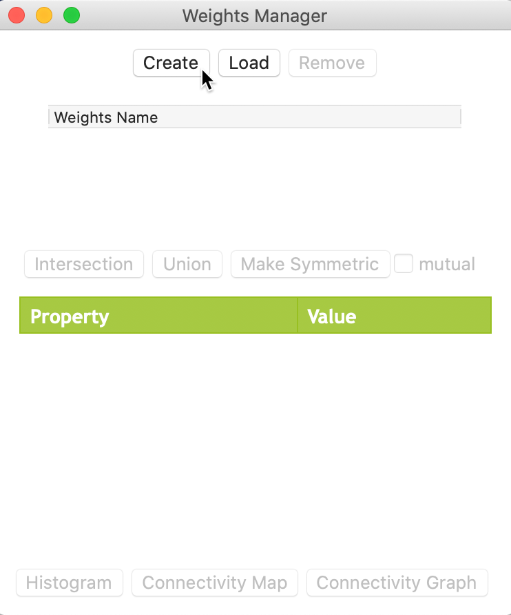
Figure 3: Weights Manager dialog

The actual construction of the weights is implemented through the Weights File Creation interface, shown in Figure 4. This provides the entry point to all the available options. Two buttons correspond to the main types of weights, based either on Contiguity or on Distance.

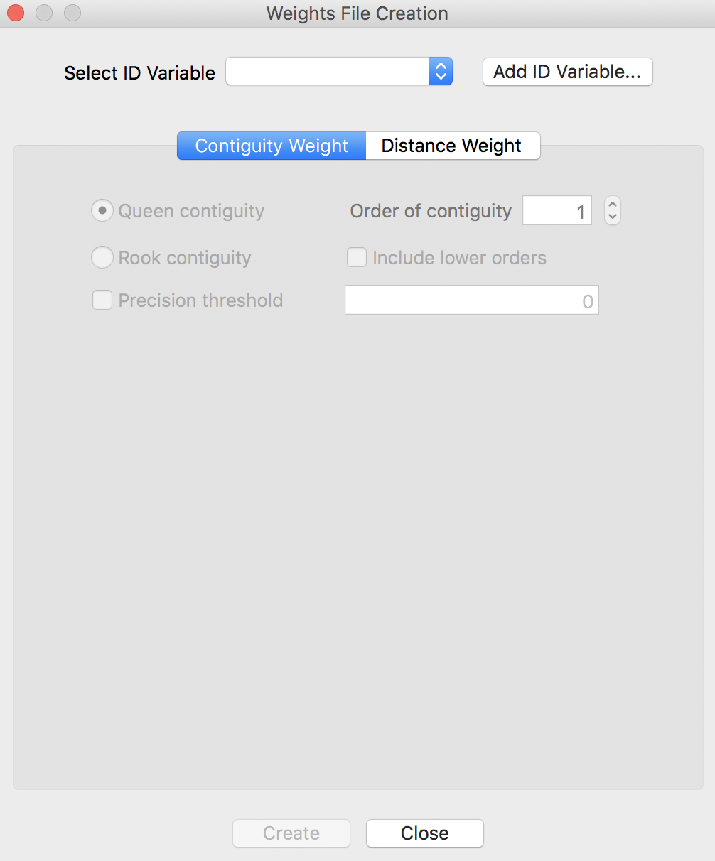
Figure 4: Weights File Creation interface

ID variable

The first item to specify is the ID Variable. This variable is a critical element to make sure that the weights are connected to the correct observations in the data table. In other words, the ID variable is a so-called key that links the data to the weights.

In GeoDa, it is best to have the ID Variable be integer. In practice, this is often not the case, and even though the identifier may look like an integer value, it is often stored as a string. For example, the standard FIPS code that comes with the U.S. county file is such a string. One way to deal with this problem is to use the Edit Variable Properties functionality in the table to turn a string into an integer, as we have seen earlier. However, sometimes there is no easy way to identify an ID variable. In that case, the Add ID Variable button provides the solution: the added ID variable is simply an integer sequence number that is added to the data table (as always, you must Save the data to make the addition permanent).

For the natregimes data set, we use FIPSNO as the ID variable, as in Figure 5. This is the county FIPS code turned into an integer value. Once the ID variable is entered, the options for the weights become available. In the opening setting, the Contiguity Weight button is active, which provides options to create queen and rook weights, as well as higher order contiguity weights. Queen contiguity with first order contiguity is set as the default, shown in Figure 5.

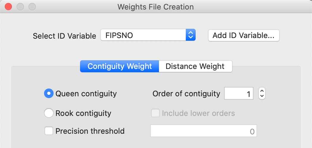
Figure 5: Weights File Creation activated

Rook contiguity

We first consider Rook contiguity, i.e., when only common sides of the polygons are considered to define the neighbor relation (common vertices are ignored). With the Rook contiguity radio button checked, as in Figure 6, a click on Create will start the weights construction process.

First, a file dialog appears in which a file name for the weights must be specified (the file extension GAL is added automatically). For example, we could use natregimes_r.gal. Since there are no real metadata in a spatial weights file, it is a good practice to make the file name something meaningful, so that you can remember what type of weight you just created. In our example, we added _r to the name of the data set to suggest rook weights. However, as we will see below, if a Project File is saved, several of the characteristics of the weights (i.e., its metadata) are stored in that file.

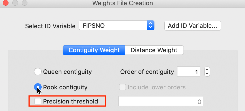
Figure 6: Rook contiguity with precision threshold option

After entering a file name and clicking on OK, the weights are computed and written to the file. At the end of this operation, a success message will appear (or an Error message if something went wrong).

Precision threshold

A useful option in the weights file creation dialog is the specification of a Precision threshold (highlighted in Figure 6). In most cases, this is not needed, but in some instances the precision of the underlying shape file is insufficient to allow for an exact match of coordinates (to determine which polygons are neighbors). When this happens, GeoDa suggests a default error band to allow for a fuzzy comparison. For example, this would be needed to create contiguity weights in the NYC sample data set.

Summary properties

After the weights are created, the weights manager becomes populated, as shown in Figure 7. The name for the file that was just created is now listed under the Weights Name. In addition, under the item Property, several summary properties are given. This includes simple descriptions, such as the type (rook), whether the weights are inherently symmetric or not (symmetric), the full file name (natregimes_r.gal), the id variable (FIPSNO), the order of contiguity (1), and the number of observations (3085).

In addition, a number of summary statistics are listed, including the minimum (1) and maximum (13) number of neighbors, the mean (5.57) and median (6) number of neighbors, and the percent nonzero cells in the matrix (0.18%). The latter is an indication of the sparsity of the weights. In the case of rook contiguity for U.S. counties, only 0.18 percent of the cells designate a neighbor relation (the rest are zeros).

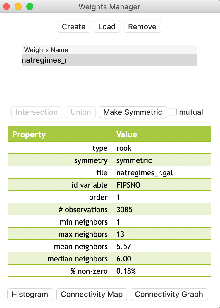
Figure 7: Rook contiguity listed in Weights Manager

GAL weights file

The GAL weights file is a simple text file that contains, for each observation, the number of neighbors and their identifiers. The format was suggested in the 1980s by the Geometric Algorithms Lab at Nottingham University and achieved widespread use after its inclusion in SpaceStat (Anselin 1992), and subsequent adoption by the R spdep package and others.

The one innovation SpaceStat added was the inclusion of a header line, with some metadata for the weights, such as the number of observations, the name of the shape file from which the weights were derived, and the name of the ID variable. As illustrated in Figure 8, for each observation, the number of neighbors is listed after its ID (e.g., for county 27077, there are 3 neighbors), followed by the IDs of the neighbors (27135 27071 27007).

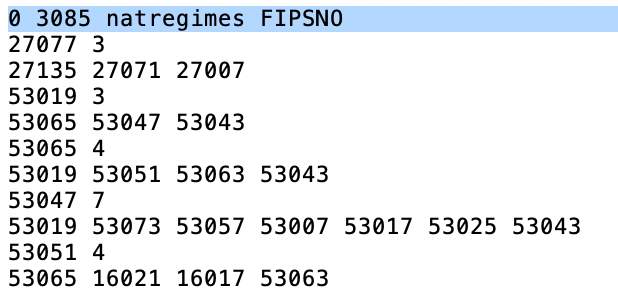
Figure 8: Contents of GAL weights file

Since the GAL file is a simple text file, it can easily be edited (e.g., to add or remove neighbors), although this is not recommended: it is easy to break the inherent symmetry of the contiguity weights.

Queen contiguity

We proceed in the same fashion to construct queen contiguity weights. The difference between the rook and queen criterion to determine neighbors is that the latter also includes common vertices. This makes the greatest difference for regular grids (square polygons), where the rook criterion will result in four neighbors (except for edge cases) and the queen criterion will yield eight. For irregular polygons (like most areal units encountered in practice), the differences will be slight. In order to deal with potential inaccuracies in the polygon file (such as rounding errors), using the queen criterion is recommended in practice. Hence it is also the default for contiguity weights.

After checking the Queen contiguity radio button, clicking on Create and entering a file name (e.g., natregimes_q.gal), the new weights will be saved to the weights file. At this point, the file name for the queen weights is included among the weights names listed in the weights manager, shown in Figure 9.

In the dialog, the highlighted weights file is the active one. This determines what weights are used in any analysis, but also drives the properties that are listed in the dialog, and what is generated by the Connectivity Histogram, Connectivity Map, and Connectivity Graph.

In the example in Figure 9, the summary properties for the queen weights are shown, since that is the highlighted weights name. The properties are almost the same as for the rook weights, except for minor differences in the maximum number of neighbors (14 vs. 13), the mean number of neighbors (5.89 vs 5.57), and the sparsity (0.19% non-zero weights compared to 0.18% for rook weights).

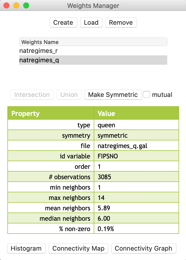
Figure 9: Queen contiguity added to weights manager

Loading weights from a file

The Weights Manager can also be used to Load weights files that are already available on disk. To start with a clean slate, we first Remove the two weights currently in the list (highlight the file name and click on Remove). Next, we select the Load button (center top) and specify the name of the weights file. In the example shown in Figure 10, we use natregimes_q as the file.

Unlike what held for the weights created on the fly in the current session, only limited descriptive items are contained in the properties list, since there are no metadata for the weights files.

In our example, GeoDa has no way of knowing whether the loaded file represents queen or rook contiguity (given as custom in the properties list), whether it is symmetric (unknown), or the order of contiguity (not listed). Therefore, it is highly recommended to use a Project File to store the weights characteristics. The descriptive statistics are computed as the file is read, so those are given as before, as shown in Figure 10.

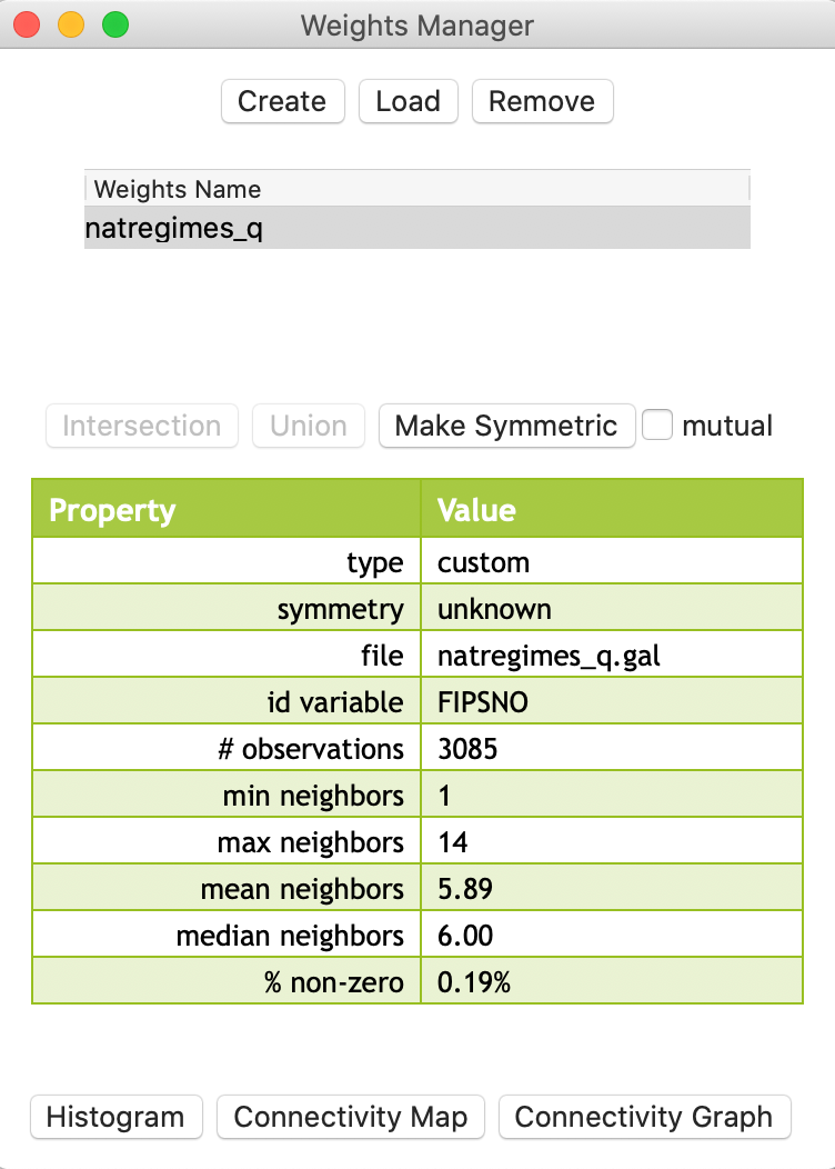
Figure 10: Loaded weights in weights manager

Weights in the Project File

Upon closing the current project, the information on the characteristics of the spatial weights is lost. When the same polygon layer is later reloaded (e.g., natregimes), each weights file has to be separately added to the project by means of the Load button in the weights manager. As illustrated in Figure 10, the summary properties listed for those loaded weights are not very informative.

A much superior alternative is to create and save a project file. This concept was introduced in the discussion of the custom category editor. The project file also contains information on the spatial weights.

In order to proceed with a project file, we first quickly re-create the rook and queen contiguity from scratch (remove any currenly listed weights that were loaded, and either use new file names, or overwrite the current files when creating the weights).

The current project information is kept in memory. As we saw earlier, it can be saved by means of the Save Project item in the File menu, as shown in Figure 11. This will prompt for a file name and save the project file with a file extension gda.

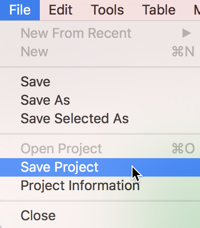
Figure 11: Save Project option

When prompted for a file name, it is best to make a selection that differentiates the current project file from the one we created for the custom categories, e.g., weights.gda.

The project file is an editable XML text file that contains all the characteristics of the spatial weights. As shown in Figure 12, the two contiguity weights created so far are included, with the properties as they were listed in the weights manager.

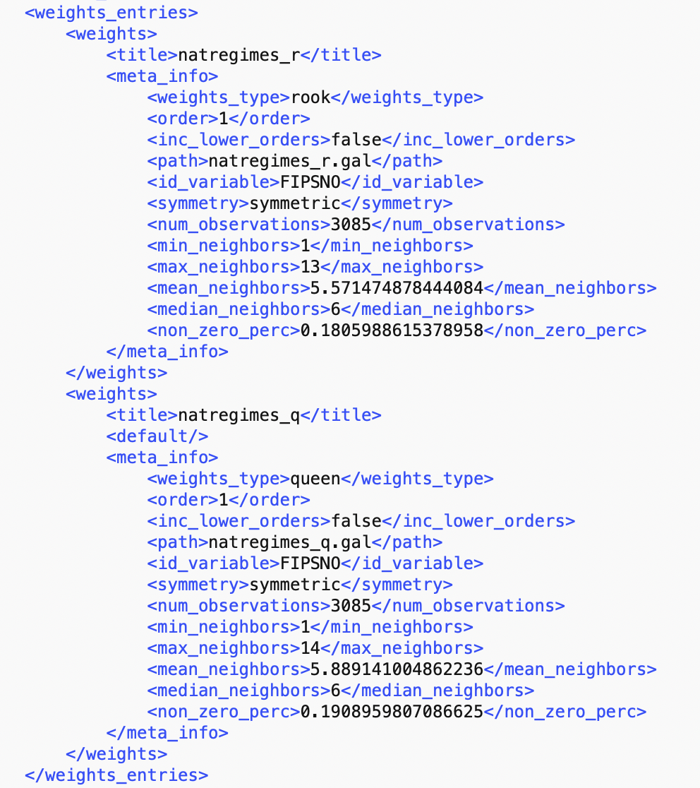
Figure 12: Weights information in project file

Once the project gda file has been saved, a new project should be started by loading the project file instead of opening a shape file (or other geographical layer). This will automatically load all the spatial weights contained in the project file and list their properties in the weights manager (in addition to custom categories, time grouped variables, etc.).

Higher Order Contiguity

Higher order contiguity weights are constructed in the same general manner as the first order weights we just covered. However, now we must specify a value larger than the default of 1 in the Order of contiguity box, as shown in Figure 13.

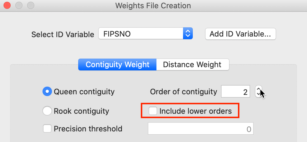
Figure 13: Higher order contiguity

As before, the weights are saved to a file after selecting the Create button and specifying a file name.

One important aspect of higher order contiguity weights is whether or not the lower order neighbors should be included in the weights structure. This is determined by a check box (highlighted in Figure 13).

Importantly, there is quite a difference between the two concepts. The pure higher order contiguity does not include any lower order neighbors. This is the notion appropriate for use in a statistical analysis of spatial autocorrelation for different spatial lag orders. In order to achieve this, all redundant and circular paths need to be removed (see Anselin and Smirnov 1996, for a technical discussion).

With the weights file as natregimes_q2.gal, the properties are listed in the weights manager shown in Figure 14.

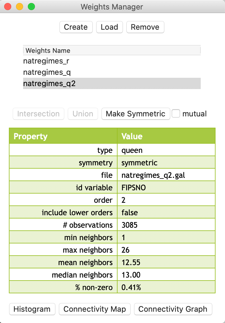
Figure 14: Second order queen weights in manager

In contrast, an encompassing notion of second order neighbors would include the first order neighbors as well. The pure second order excludes these, even though there are two steps – back and forth – connecting each observation to its first order neighbor. However, as mentioned, to avoid redundancy, these are excluded.

The notion of inclusive increasing orders of contiguity side steps the redundancy issue, since both first and second neighbors are included. This can be used in a way similar to increasing distance bands, i.e., bands increasing by order of contiguity.

We also create the inclusive second order type queen contiguity weights, now with the box checked and with file name natregimes_q2i.gal. Its characteristics are listed in the weights manager, shown in Figure 15.

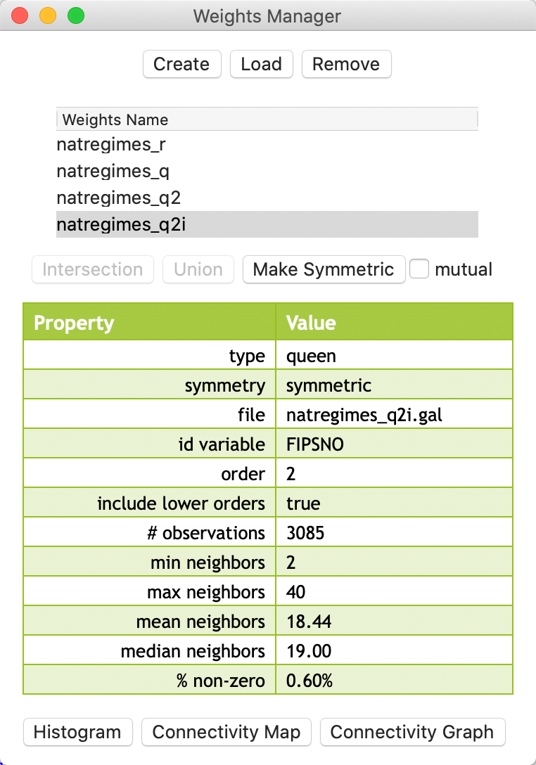
Figure 15: Inclusived second order weights in manager

The difference between the two concepts can be easily gathered from the descriptive statistics. As expected, the inclusive second order weights are denser, as illustrated by the mean and median number of neighbors (respectively 18.44 compared to 12.55; and 19 compared to 13), and the percent non-zero (0.60% compared to 0.41%).

Weights Characteristics

Some useful characteristics of the currently selected weights are provided in the Weights Manager by means of the Connectivity Histogram, the Connectivity Map, and the Connectivity Graph. To continue, we should have at least the queen contiguity weights available in the weights manager.

Connectivity histogram

The Histogram button at the left-hand side of the bottom of the weights manager produces a connectivity histogram. This shows the number of observations for each value of the cardinality of neighbors (i.e., how many observations have the given number of neighbors). The graph, illustrated in Figure 16 for the queen contiguity associated with the U.S. counties, is a standard GeoDa histogram, with a number of options available, some of which are generic, and some specific to the connectivity histogram.

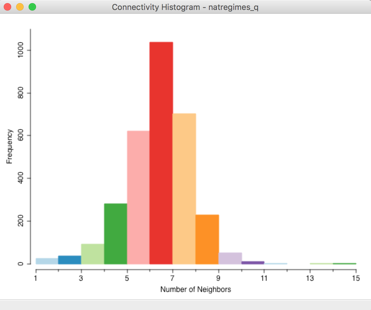
Figure 16: Connectivity histogram - queen weights

The overall pattern is quite symmetric, with a mode of 6 (i.e., most counties have 6 neighbors). In addition to the visual inspection, the usual statistics of the distribution can be added to the bottom of the table by means of the View > Display Statistics option, in Figure 17.

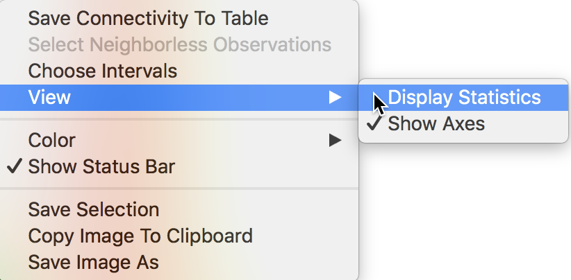
Figure 17: Display connectivity statistics

From the descriptive statistics listed at the bottom of the graph in Figure 18, we can see that the median number of neighbors is 6, the average is 5.89, and the maximum is 14. This matches the descriptive statistics listed in the properties of the weights manager. In addition, the number of observations in each interval is listed as well.

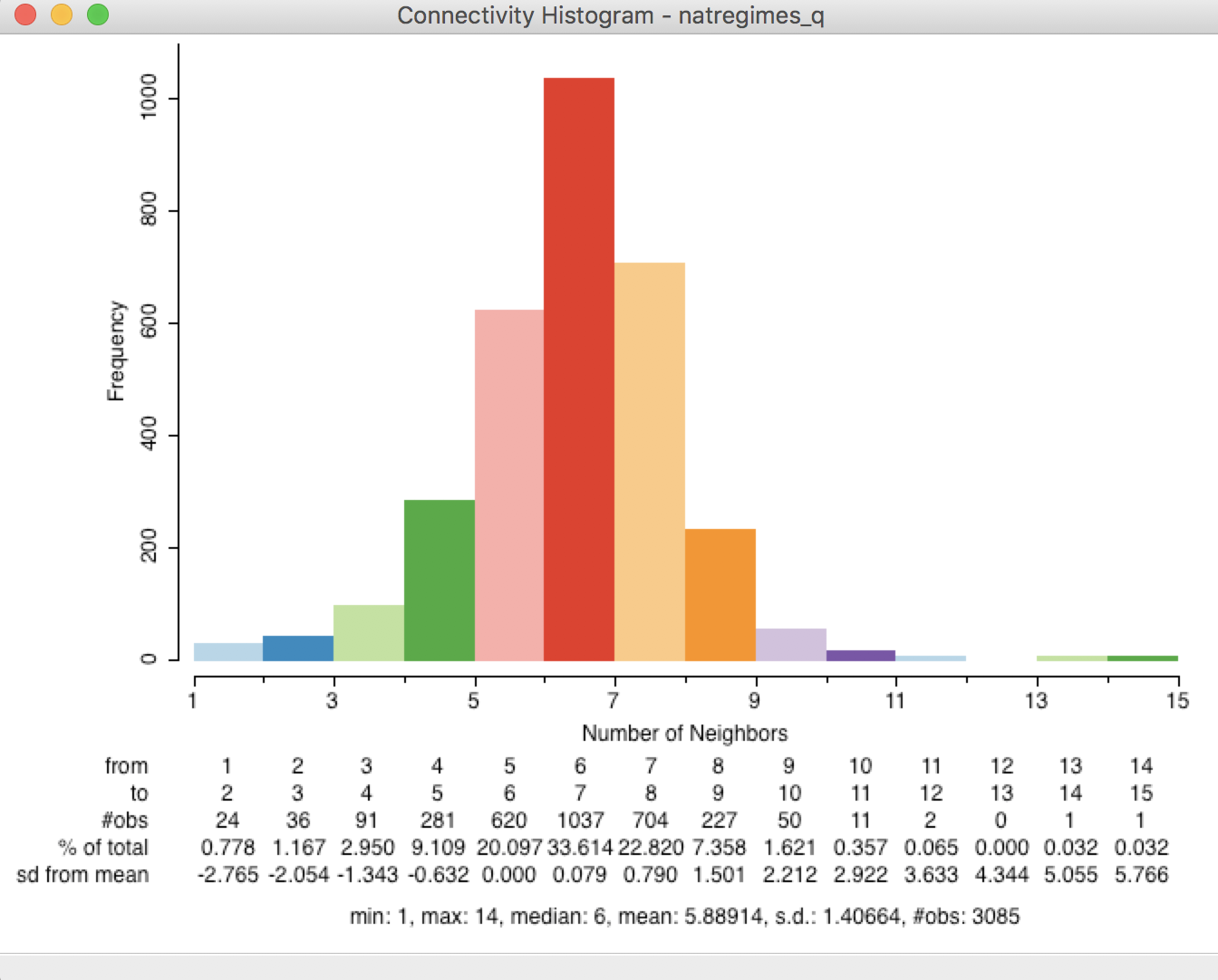
Figure 18: Connectivity histogram with statistics

In standard GeoDa fashion, the connectivity histogram is connected to all the other views through linking and brushing. For example, as shown in Figure 19, by selecting the modal bar, all 1037 counties with six neighbors are highlighted in the U.S. county map.

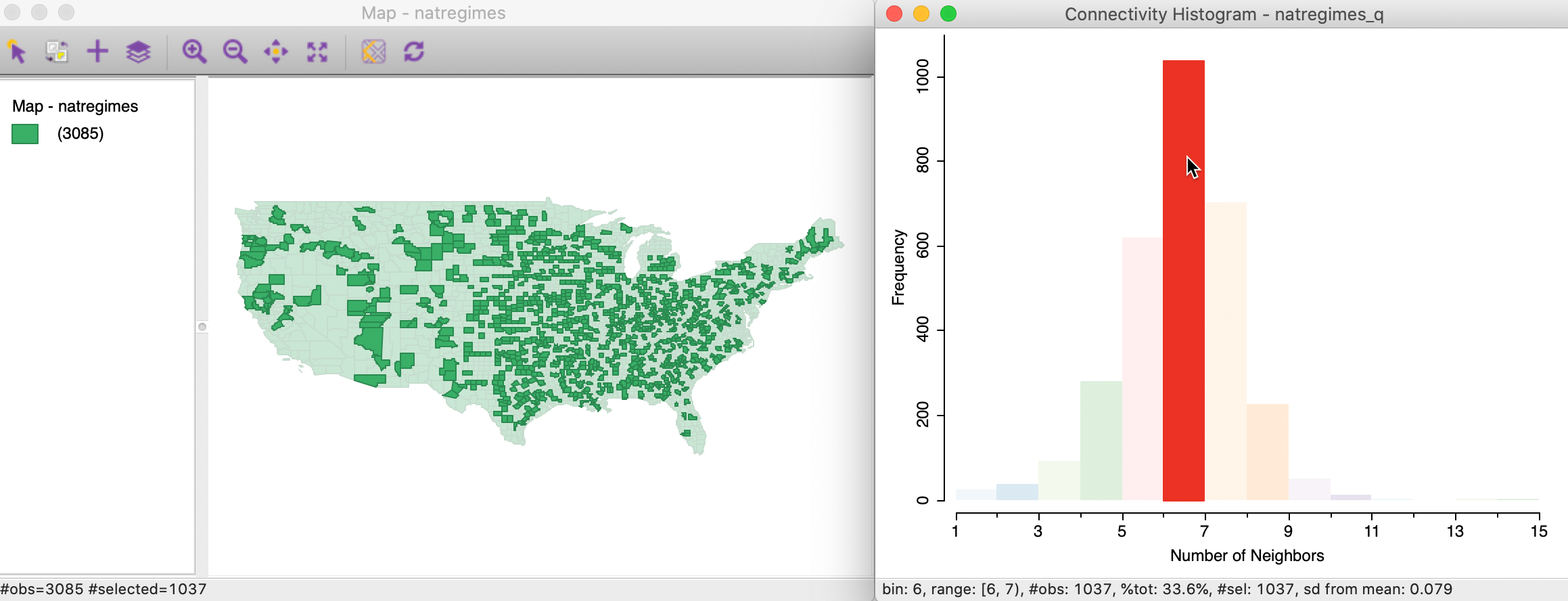
Figure 19: Counties with six neighbors

In addition, we can check the correspondence between queen and rook contiguity. The selected observations with six neighbors according to the queen criterion are highlighted in the connectivity histogram for rook as well, as in Figure 20. This illustrates how 30 counties that had six neighbors in queen contiguity (the selected observations go from 1037 to 1007 for six neighbors in rook) have fewer neighbors according to rook contiguity (we see their distribution spread over four and five neighbors).

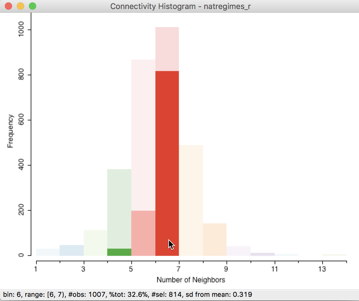
Figure 20: Counties with six queen neighbors in rook histogram

It is good practice to check the connectivity histogram for any “strange” patterns, such as observations with only one neighbor and neighborless observations (isolates). The latter will be covered in the discussion of distance-based weights.

Ideally, we like the distribution of the cardinalities to be nice and symmetric, with a limited range. We are on the lookout for bimodal distributions (some observations have few neighbors and some many) and other deviations from symmetry.

Saving the neighbor cardinality to the table

A useful option of the connectivity histogram is to save the neighbor cardinality to the data table as an additional column/variable to be used in further analysis. The Save Connectivity to Table option is invoked in the usual way by right clicking on the histogram view, which yields the menu shown in Figure 21.

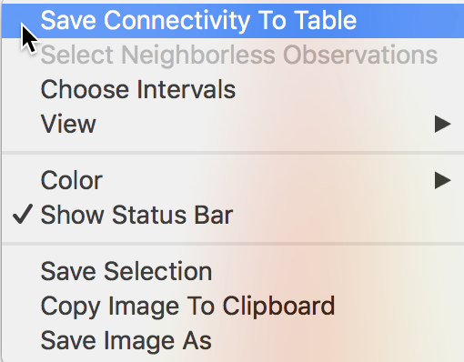
Figure 21: Save connectivity to table

After selecting the option, a small dialog appears in which the name for the new variable can be specified. The default, shown in Figure 22, is a generic NUM_NBRS, which may not be the most insightful when different spatial weights are being compared. For now, we keep the variable name as is.

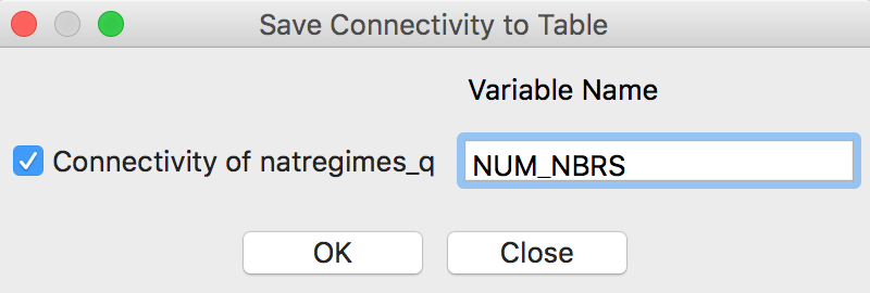
Figure 22: Variable for neighbor cardinality

Upon clicking OK, an additional column is added to the data table in Figure 23. This lists the number of neighbors for that observation for the particular spatial weights specification that was used for the connectivity histogram. The number of neighbors is an important input into the calculation of the significance of the local join count statistic, covered in a later chapter.

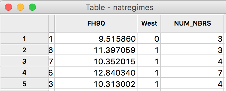
Figure 23: Cardinality added to table

Connectivity map

The middle button at the bottom of the Weights Manager interface (e.g., see Figure 9) brings up a Connectivity Map. This is a standard GeoDa map view (with all the usual map features invoked through toolbar icons, including zooming and panning), but with a special functionality that highlights the neighbors of any selected observation.

In our example, using queen contiguity, this starts with the usual green themeless map of all the U.S. counties, with the name of the matching spatial weights file listed in the window header (here, natregimes_q), as in Figure 24.

As soon as the pointer is moved over one of the observations, it is selected and its neighbors are highlighted. Note that this behavior is slightly different from the standard selection in a map, since it does not require a click to select. Instead, the pointer is in so-called hover mode. As soon as the pointer moves outside the main map, the whole country is shown again.

In Figure 24, the pointer is over Coconino county, AZ. The county is selected (the other counties become transparent) and the outlines of the neighboring counties are shown. Its ID (FIPSNO=4005) and the IDs of the six neighbors are shown in the status bar (49037, 49025, 4017, 4015, 4025, and 4007). The ID values shown in the status bar match the ID variable selected for the spatial weights. This is different from the behavior in a generic map, where the simple observation sequence number is shown only for the selected observations (not the neighbors).

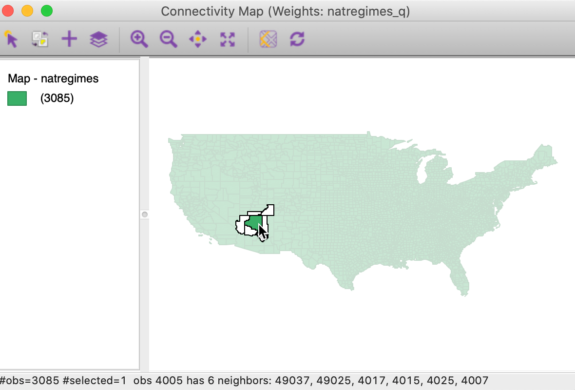
Figure 24: Connectivity map – Coconino county AZ selected

The Connectivity Map allows us to investigate strange patterns in the neighbor structure for some counties. For example, several counties in the state of Virginia are so-called city counties, surrounded by a larger area county. Zooming in on Charlotsville, VA (fipsno=51540) illustrates this phenomenon, as shown in Figure 25.

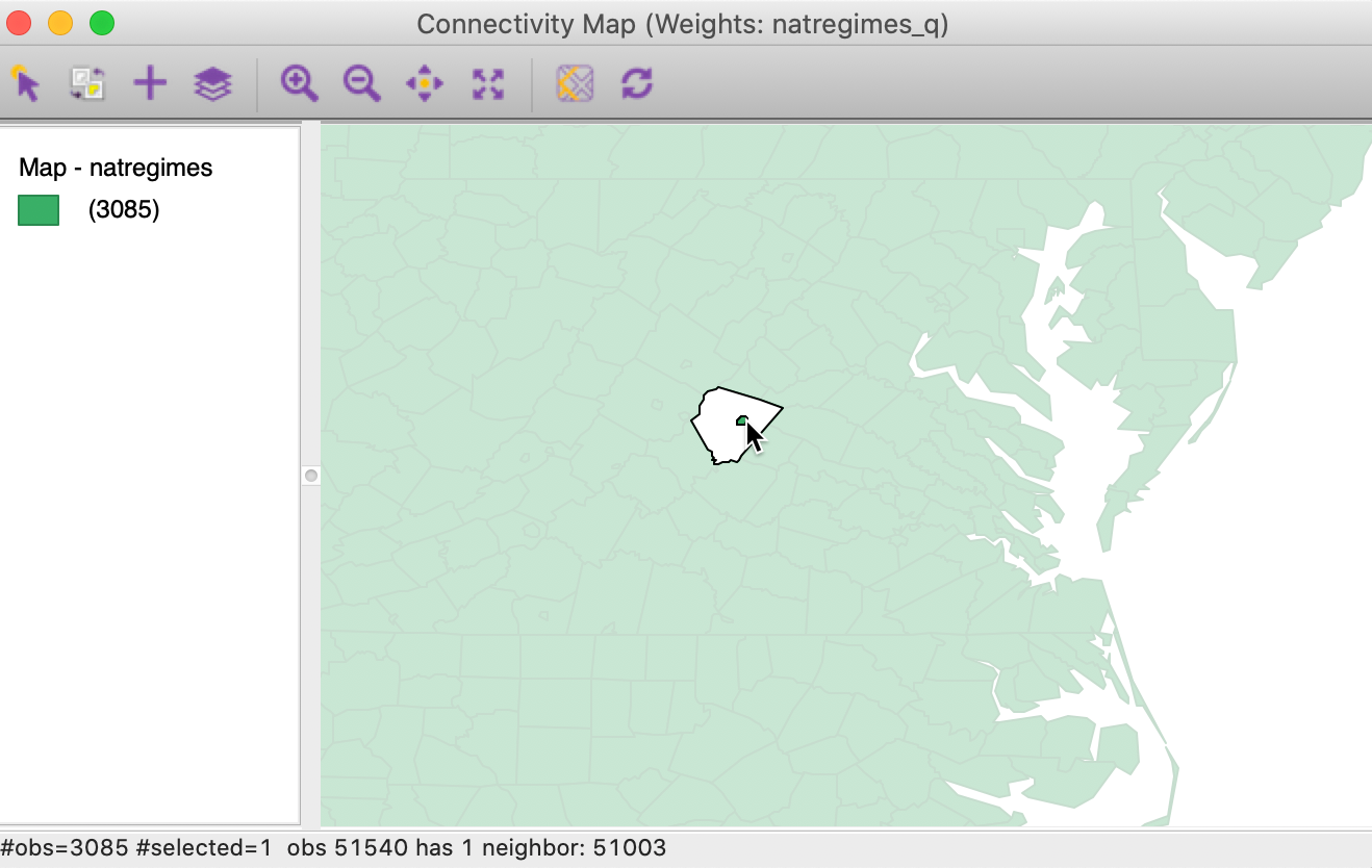
Figure 25: Neighbors for Charlotsville, VA

The sole neighbor of Charlotsville is Albermarle county (fipsno=51003), which itself has nine neighbors, including Charlotsville, as indicated by the tiny outline within its polygon, shown in Figure 26.

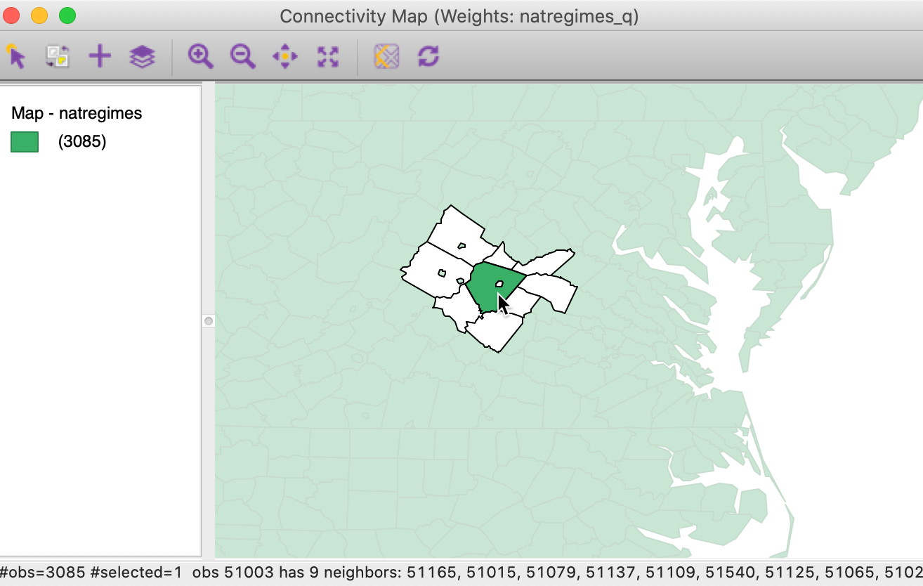
Figure 26: Neighbors for Albermarle, VA

Connectivity map options

Close examination of the neighbor structure depicted in Figure 26 might suggest an inconsistency. The status bar mentions nine neighbors, but counting the polygons would imply 12, when including the small islands within the larger neighboring counties. However, in fact, these city-counties are not actual neighbors. In the map, they are rendered in a slightly different shade (the same transparent green as the other not selected counties) than the white for the neighbors, but it is difficult to distinguish.

To highlight the contrast, the shading of the neighbors should be changed. The Connectivity item in the list of map options contains a number of ways to adjust the fill and outline color of the neighbors and the selection, as listed in Figure 27.

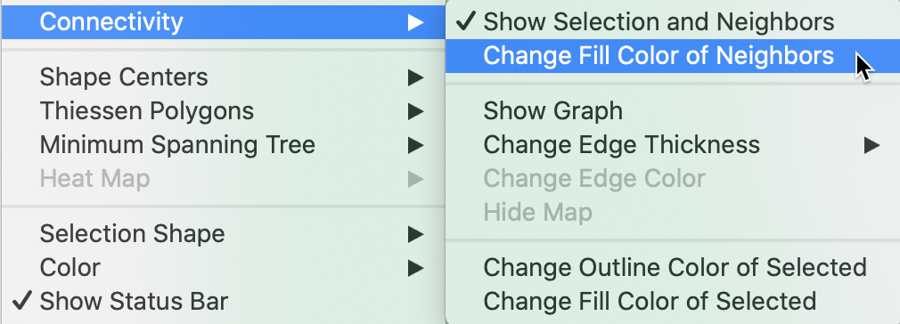
Figure 27: Neighbor fill color option

For example, changing the fill color for the neighbors to red results in the selection as depicted in Figure 28. Now it is clear that there are only nine red polygons that correspond to the neighbors of the selection.

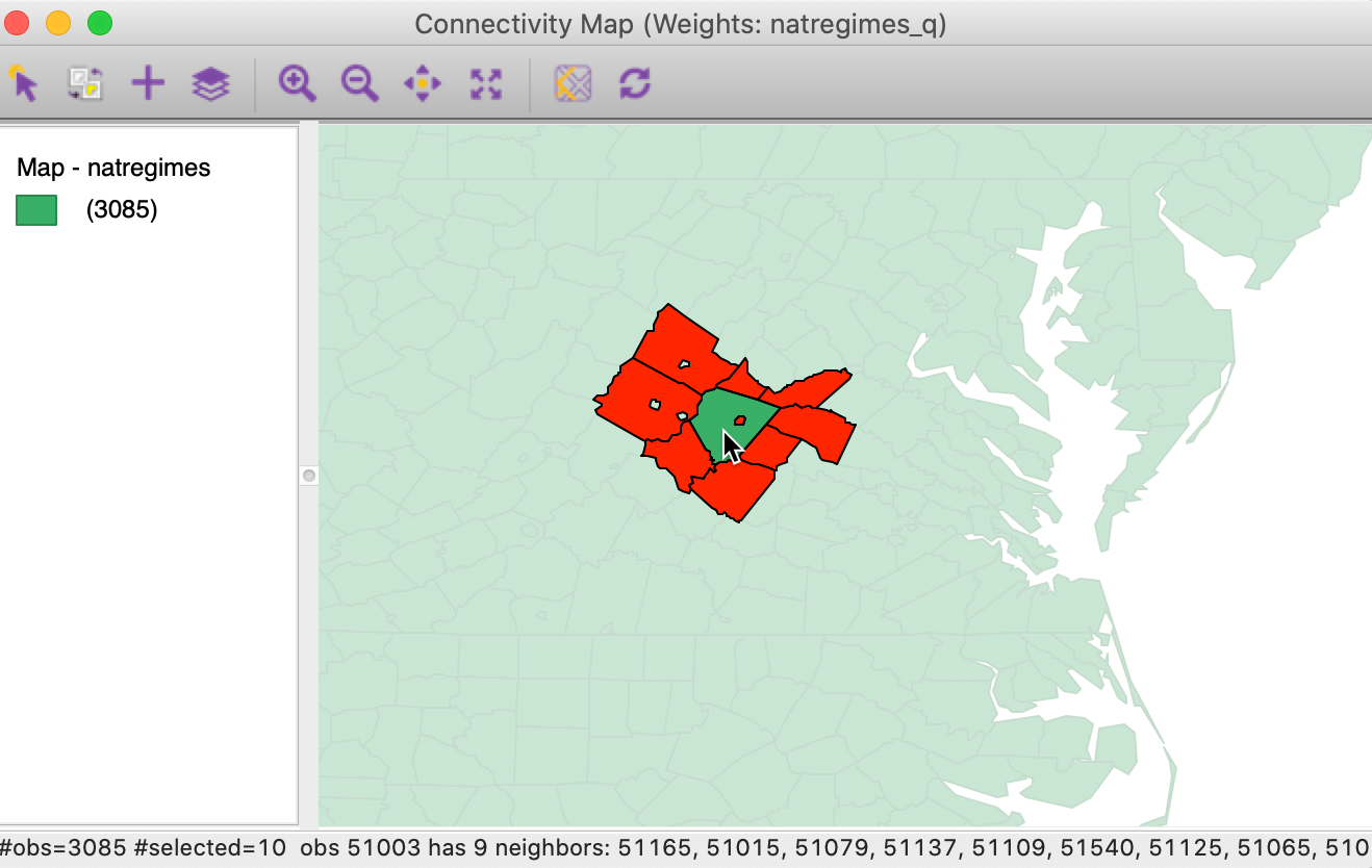
Figure 28: Neighbor fill with red color option

Connectivity graph

The right-most button at the bottom of the Weights Manager interface (e.g., see Figure 9) brings up a Connectivity Graph. Like the Connectivity Map, this is a standard GeoDa map view, with all the usual map features invoked through toolbar icons, including zooming and panning.

In this map, the graph structure that corresponds to the spatial weights connectivity is superimposed on the map. For the U.S. counties as a whole, using queen contiguity, this view tends to be somewhat cluttered, as in Figure 29. As for the Connectivity Map, the window header lists the corresponding spatial weights file (here, again, natregimes_q).

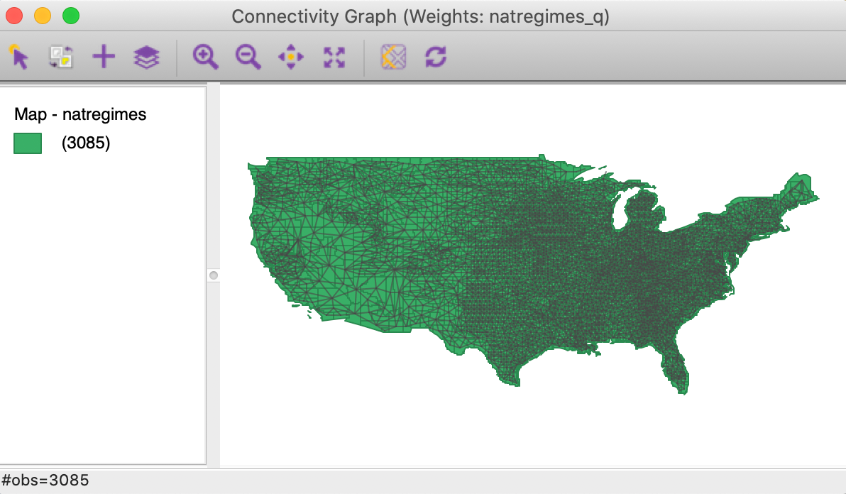
Figure 29: Connectivity graph - US counties

All the standard map options work in the usual way. For example, we could zoom in on the Southwest and select Coconino county in Arizona, as in Figure 30. The selection removes the graph structure for the other counties from the map, but shows the selected county and its neighbors, connected by the edges in the graph.

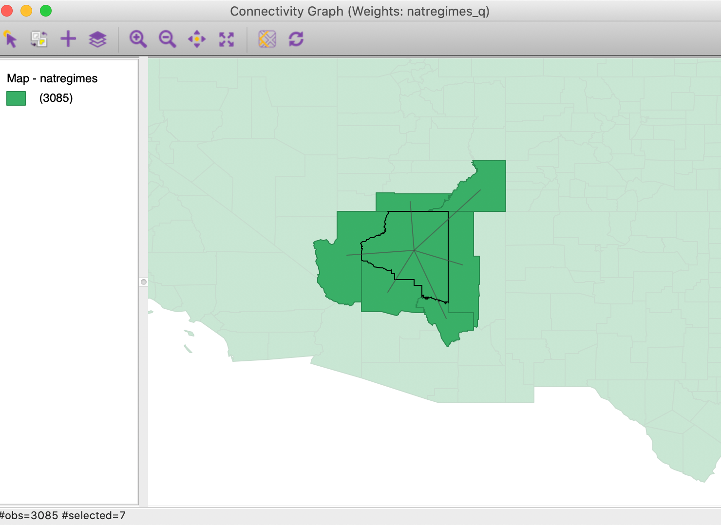
Figure 30: Connectivity graph - Coconino county, AZ

Connectivity graph options

As in the connectivity map, there are a few options that allow us to customize the representation of the graph structure, listed in Figure 27. These include the color and thickness of lines, and whether the background map is shown or not.

The default edge thickness is Normal, but two other options are available, to make the lines thicker (Strong) or thinner (Light). It is also often useful to change the color of the graph to something different from the default black.

The most dramatic of the options is the Hide Map feature. By selecting this, the background map is removed and only the pure graph structure remains, as in Figure 31. Unchecking this options brings the map back.

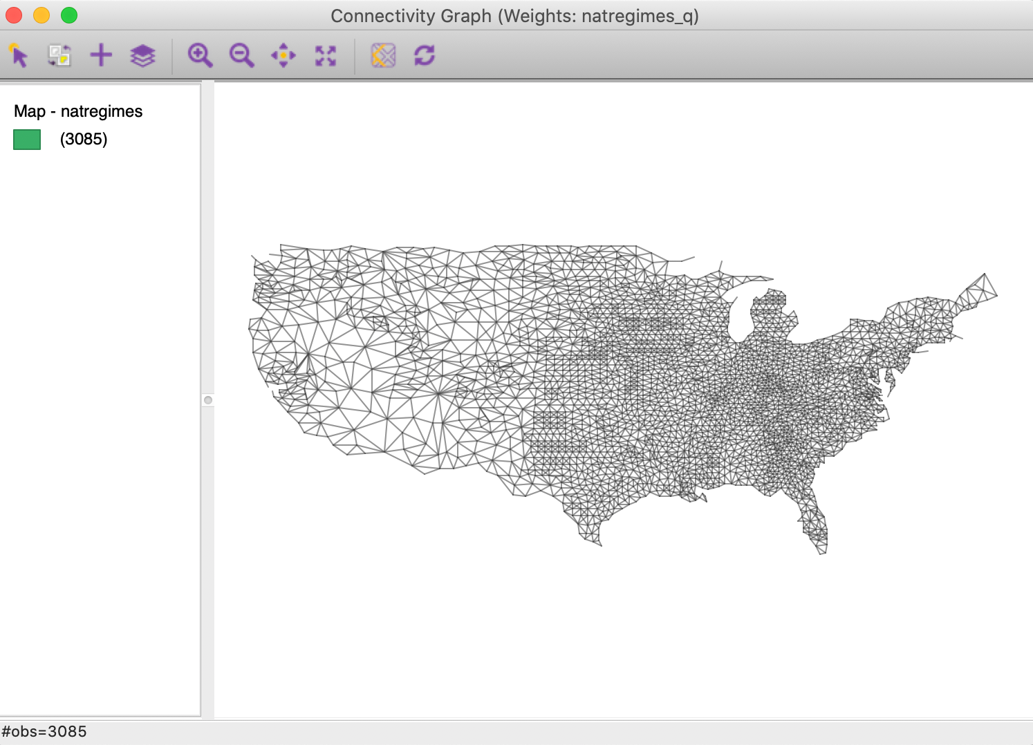
Figure 31: Connectivity graph without background map

Connectivity Option

Connectivity Option in the Map

With an active weights matrix, the Connectivity item in the map options menu becomes active. This provides functionality similar to that in a Connectivity Map, but applied to any current map.

The functionality is invoked by selecting Connectivity > Show Selection and Neighbors from the options menu, as in Figure 32.

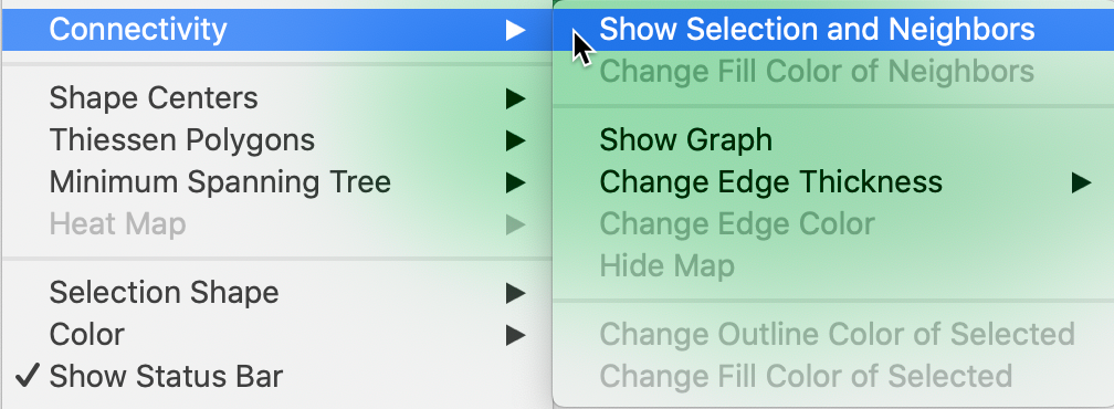
Figure 32: Show selection and neighbors option

With this option checked, the selection feature works the same as in the Connectivity Map, as illustrated in Figures 24 to 26. The main difference between the functionality in the Connectivity Map and the Connectivity option in any thematic map is that the latter is updated to the current active spatial weights file. In contrast, when selecting the Connectivity Map from the weights manager, there is only one such map, tied directly to the weights file from which it was invoked.

With the Show Selection and Neighbors option checked, it becomes possible to Change Outline Color of Neighbors, and to Change Fill Color of Neighbors, in the same way as illustrated for the connectivity map.

Connectivity Option in the Table

Neighbors of selected observations can also be displayed by means of a a feature of the table Selection Tool, as long as a weights matrix is active.

To illustrate this, we first select Coconino county in a generic themeless map (with the Show Selection and Neighbors option turned off). The view is as in Figure 33.

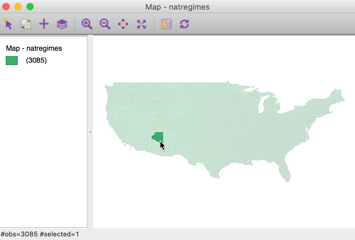
Figure 33: Coconino county selected in themeless map

The Selection Tool is activated in the usual way by right clicking anywhere in the table. The Add Neighbors to Selection button is central in the middle panel of Figure 34. Note that the Weights must be specified and there has to be an active selection. By default, the drop-down list will show the currently active weights, i.e., natregimes_q in our example.

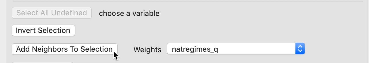
Figure 34: Adding neighbors to selection

Clicking on the button will add the neighbors of Coconino county to the map, as in Figure 35.

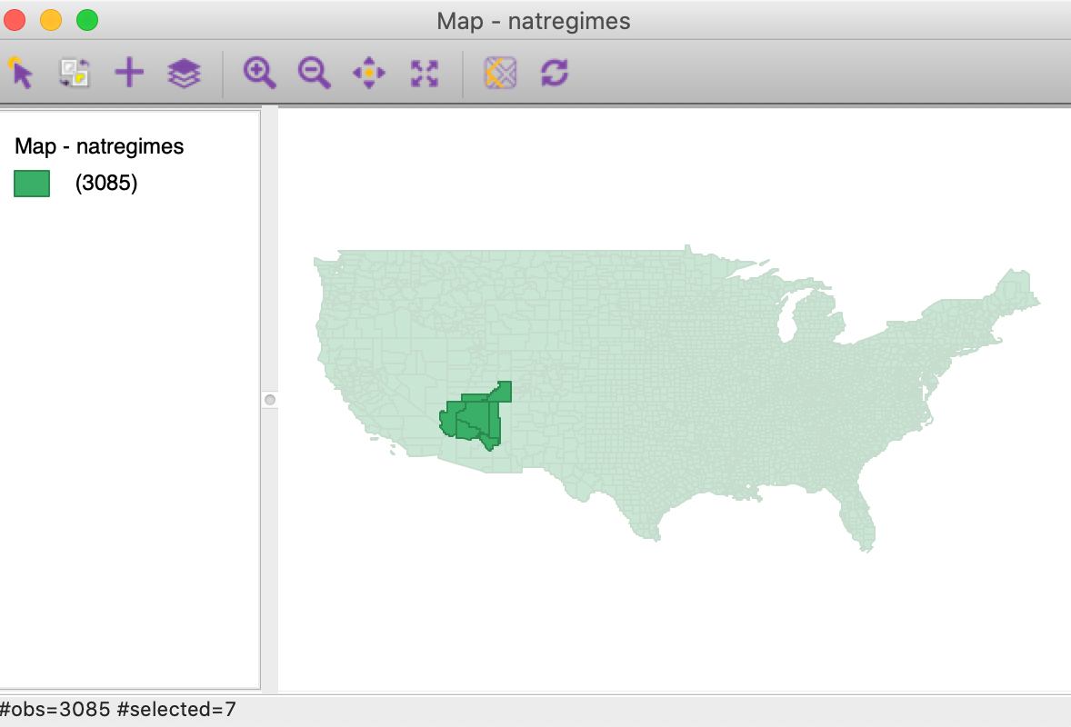
Figure 35: Coconino county with neighbors

References

Anselin, Luc. 1992. SpaceStat, a Software Program for Analysis of Spatial Data. National Center for Geographic Information; Analysis (NCGIA), University of California, Santa Barbara, CA: National Center for Geographic Information; Analysis (NCGIA).

Anselin, Luc, and Sergio J. Rey. 2014. Modern Spatial Econometrics in Practice, a Guide to Geoda, Geodaspace and Pysal. Chicago, IL: GeoDa Press.

Anselin, Luc, and Oleg Smirnov. 1996. “Efficient Algorithms for Constructing Proper Higher Order Spatial Lag Operators.” Journal of Regional Science 36: 67–89.

---

1. University of Chicago, Center for Spatial Data Science – anselin@uchicago.edu↩︎

2. An exception to this rule are the diagonal elements in kernel-based weights, which are considered in a later chapter.↩︎

3. Strictly speaking, this is only correct in the absence of so-called isolates, i.e., observations without neighbors. With \(q\) isolates, the sum \(S_0 = n - q\).↩︎

4. A third notion, referred to as bishop contiguity, is based on the existence of common vertices between two spatial units. It is seldom used in practice, and has not been implemented in GeoDa.↩︎

GeoDa is maintained by lixun910. This page was generated by GitHub Pages using the Cayman theme by Jason Long.