Local Spatial Autocorrelation (3)

Multivariate Local Spatial Autocorrelation

Introduction

In this chapter, we cover the extension of the concept of local spatial autocorrelation to the multivariate domain. This turns out to be particularly challenging due to the difficulty in separating pure attribute correlation among multiple variables from the spatial effects.

We consider three methods. First, we discuss a bivariate version of the Local Moran, which is useful in a space-time context, but needs to be interpreted with great caution in pure cross-sectional settings. We next outline an extension of the Local Geary statistic to the multivariate Local Geary. We close with a discussion of a recently introduced local neighbor match test.

As in the previous Chapter, we continue to use both the natregimes and the Guerry data sets to illustrate these methods.

Objectives

• Understand the issues related to extending a spatial autocorrelation measure to a multivariate setting

• Identify clusters and outliers with the bivariate extensions of the Local Moran statistic

• Identify clusters and outliers with the Multivariate Local Geary

• Understand the issues pertaining to interpreting the results of the multivariate Local Geary

• Identify clusters by means of the local neighbor match test

GeoDa functions covered

• Space > Bivariate Local Moran’s I
• Space > Multivariate Local Geary
• Space > Local Neighbor Match Test

Preliminaries

As in the previous Chapter, we will continue to use both the Guerry data set and the natregimes data set. For each of these, we need an active spatial weights matrix, e.g., guerry_85_q for the former and natregimes_q for the latter. See the description in earlier Chapters on how to accomplish this.

Also, as in the previous Chapter, we need some further preparation of the natregimes data set to make the variables time sensitive. If not done so already, we need to use the Time Editor to group the homicide rates hr60 through hr90 into the variable hr (we do not need the count variables in this Chapter).

The Multivariate Spatial Autocorrelation Problem

Designing a spatial autocorrelation statistic in a multivariate setting is fraught with difficulty. The most common statistic, Moran’s I, is based on a cross-product association, which is the same as a bivariate correlation statistic. As a result, it is difficult to disentangle whether the correlation between multiple variables at adjoining locations is due to the correlation among the variables, or a similarity due to being neighbors in space.

Early attempts at extending Moran’s I to multiple variables focused on principal components, as in the suggestion by Wartenberg (1985), and later work by Dray, Saïd, and Débias (2008). However, these proposals only dealt with a global statistic. A more local perspective along the same lines is presented in Lin (2020), although it is primarily a special case of a geographically weighted regression, or GWR (Fotheringham, Brunsdon, and Charlton 2002).

Lee (2001) outlined a way to separate a bivariate Moran-like spatial correlation coefficient into a spatial part and a Pearson correlation coefficient. However, this relies on some fairly strong simplifying assumptions that may not be realistic in practice.

In Anselin (2019), the idea is proposed to focus on the distance between observations in both attribute and geographical space and to construct statistics that assess the match between those distances. In general, the squared multi-attribute distance between a pair of observations \(i, j\) on \(k\) variables is given as: \[d_{ij}^2 = || x_i - x_j || = \sum_{h=1}^k (x_{ih} - x_{jh})^2,\] with \(x_i\) and \(x_j\) as vectors of observations. In some expressions, the squared distance will be preferred, in others, the actual distance (\(d_{ij}\), its square root) will be used. The overall idea is to identify observations that are both close in multiattribute space and close in geographical space.

First, we consider a simple bivariate extension of the Local Moran, which is not based on the distance measures.

Bivariate Local Moran

Principle

The treatment of the bivariate Local Moran’s I closely follows that of its global counterpart (see also Anselin, Syabri, and Smirnov 2002). In essence, it captures the relationship between the value for one variable at location \(i\), \(x_i\), and the average of the neighboring values for another variable, i.e., its spatial lag \(\sum_j w_{ij} y_j\). Apart from a constant scaling factor (that can be ignored), the statistic is the product of \(x_i\) with the spatial lag of \(y_i\) (i.e., \(\sum_j w_{ij}y_j\)), with both variables standardized, such that their means are zero and variances equal one:

\[ I_{i}^B = c x_i \sum_j w_{ij} y_j,\] where \(w_{ij}\) are the elements of the spatial weights matrix.

As is the case for its global counterpart, this statistic needs to be interpreted with caution, since it ignores in-situ correlation between the two variables (see the discussion of global bivariate spatial autocorrelation for details).

A special case of the bivariate Local Moran statistic is comparing the same variable at two points in time. The most meaningful application is where one variable is for time period \(t\), say \(z_t\), and the other variable is for the neighbors in the previous time period, say \(z_{t-1}\). This formulation measures the extent to which the value at a location in a given time period is correlated with the values at neighboring locations in a previous time period, or an inward influence. It is illustrated in the example below.

An alternative view is to consider \(z_{t-1}\) and the neighbors at the current time. This would measure the correlation between a location and its neighbors at a later time, or an outward influence. The first specification is more accepted, as it fits within a standard space-time regression framework.

Implementation

The bivariate Local Moran functionality is invoked from the first group in the Cluster Maps toolbar icon, as show in Figure 1, or from the menu as Space > Bivariate Local Moran’s I.

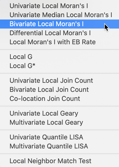
Figure 1: Bivariate Local Moran from the toolbar

Next, we proceed in the usual fashion by selecting a variable for \(x\), for example hr(90), and a variable for \(y\), say hr(80), in the variable selection dialog, shown in Figure 2. Since the variables are time enabled, the proper period is selected by means of the Time drop down list. Also note that the spatial weights matrix has been set to natregimes_q.

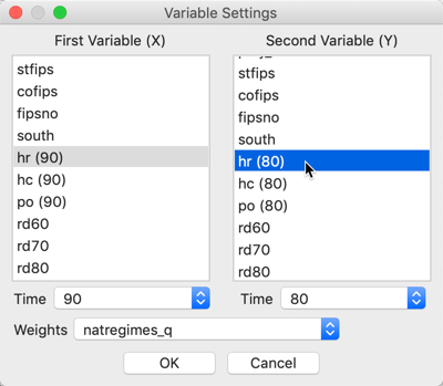
Figure 2: Bivariate Local Moran variable selection

The next prompt gives the familiar choice of a Significance Map, Cluster Map, and Moran Scatter Plot, with just the Cluster Map selected as the default. With the default setting, the result is based on 999 permutations with a p-value of 0.05, as shown in Figure 3.

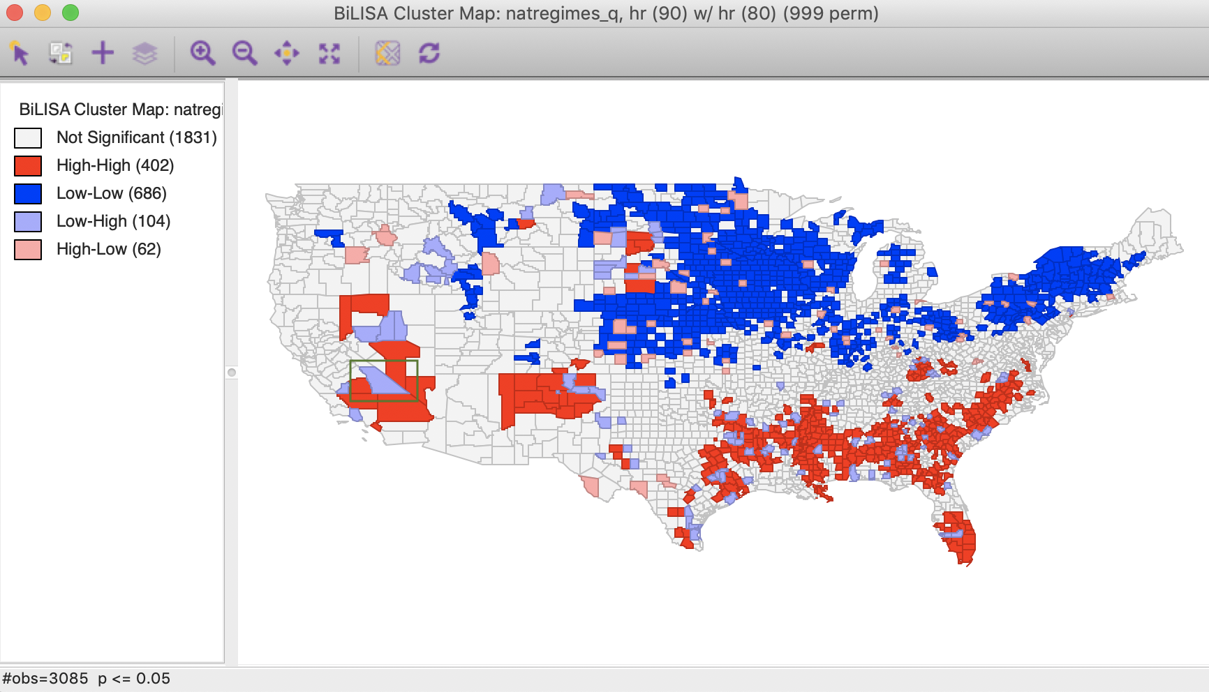
Figure 3: Bivariate Local Moran cluster map

All the options for randomization, significance filter, and saving the results are the same as for the univariate Local Moran and will not be further discussed here.

Interpretation

As mentioned, the interpretation of the bivariate Local Moran cluster map warrants some caution, since it does not control for the correlation between the two variables at each location (i.e., the correlation between \(x_i\) and \(y_i\)). To illustrate this issue, consider the space-time case, where one can interpret the results of the High-High and Low-Low clusters in Figure 3 as locations where high/low values at time \(t\) (in our example, homicide rates in 1990) were surrounded by high/low values at time \(t -1\) (homicide rates in 1980) more so than would be the case randomly. This could either be attributed to the surrounding locations in the past affecting the central location at the current time (a form of a diffusion effect), but could also be due to a strong inertia, in which case there would be no diffusion. More precisely, if the homicide rates in all locations are highly correlated over time, then if the surrounding values in \(t - 1\) were correlated with the value at \(i\) in \(t - 1\), then they would also tend to be correlated with the value at \(i\) in \(t\) (through the correlation between \(y_{j,t-1}\) and \(y_{j,t}\)). Hence, while these findings could be compatible with diffusion, this is not necessarily the case. The same complication affects the interpretation of the bivariate Local Moran coefficient between two variables at the same point in time.

To illustrate the problems with interpreting bivariate local cluster maps, we take the case of spatial outliers. In addition to the bivariate results, we also consider the univariate Local Moran cluster maps for the variable in each time period, i.e., in \(t - 1\) and in \(t\), i.e., hr(80) and hr(90), as shown in Figures 4 and 5.

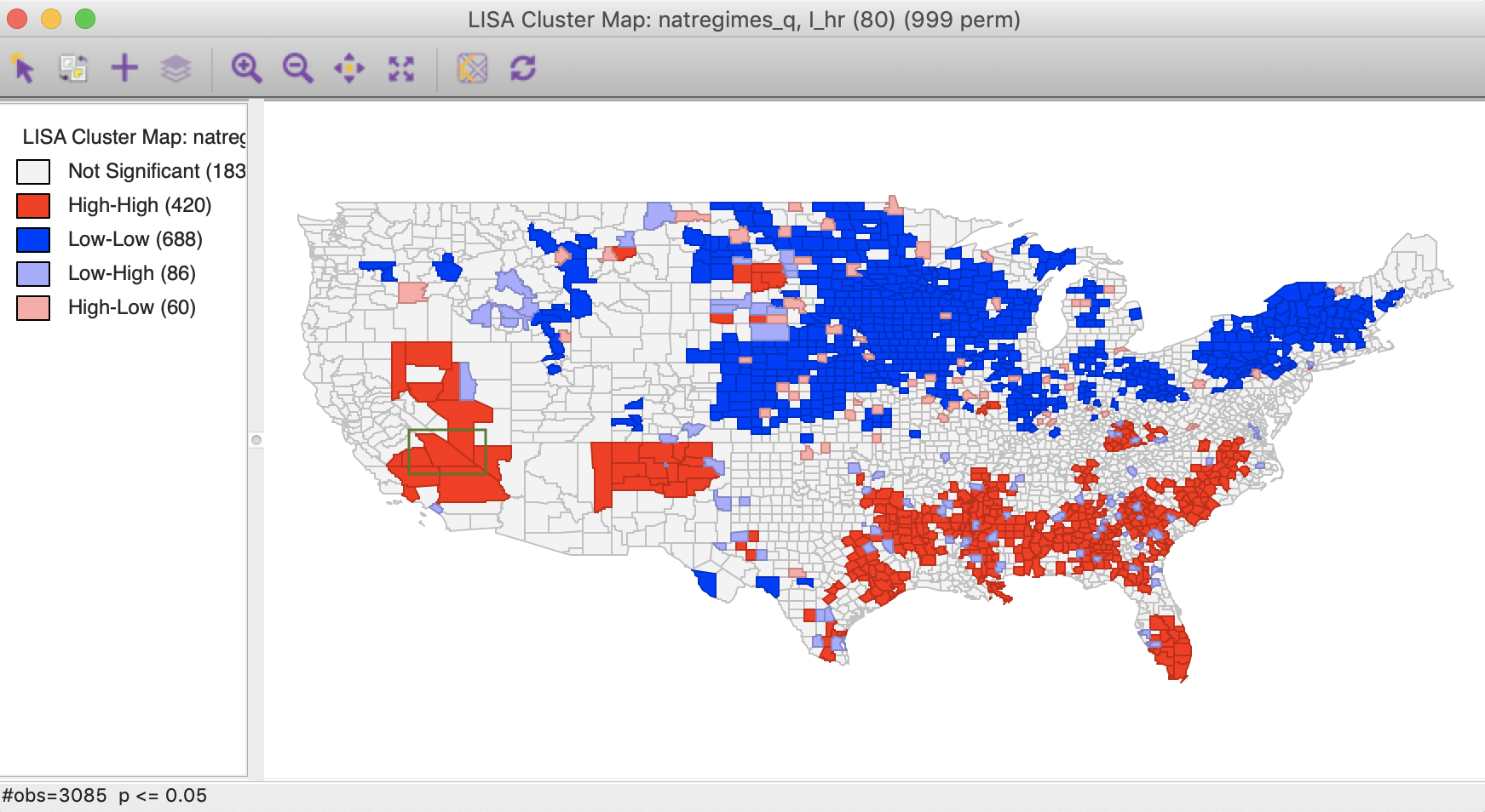
Figure 4: Local Moran cluster map – hr80

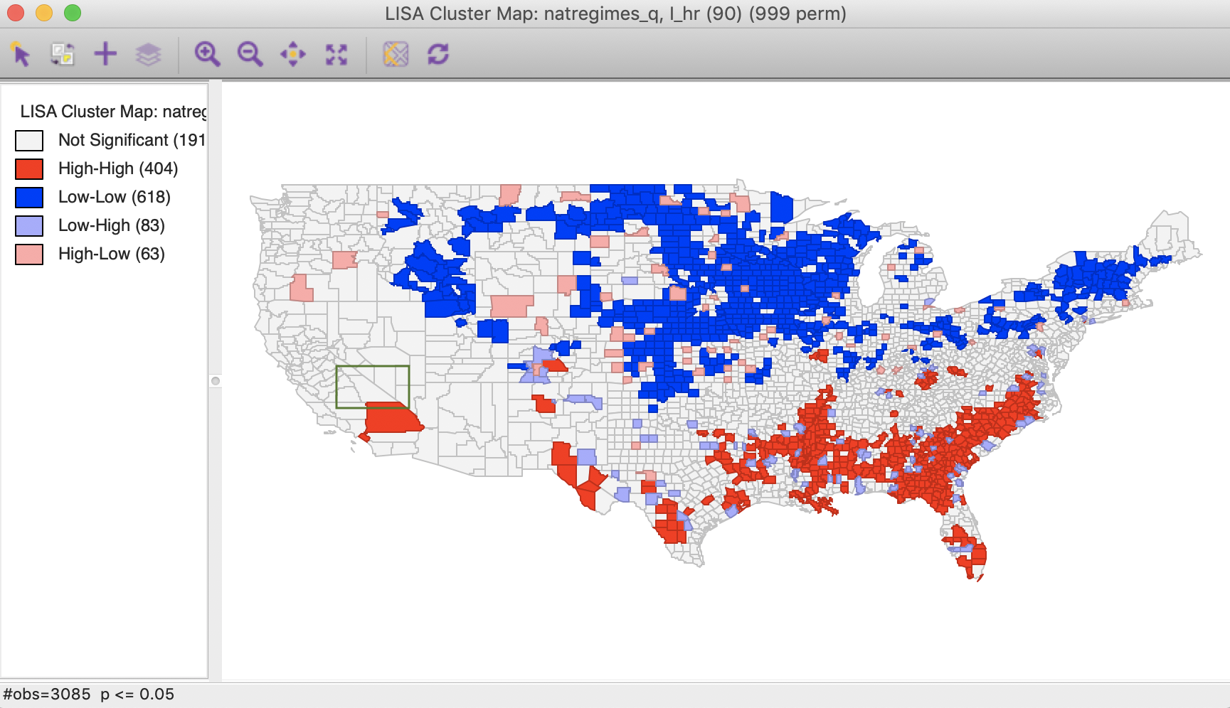
Figure 5: Local Moran cluster map – hr90

The highlighted county is Inyo county (CA), which is identified as a Low-High spatial outlier in Figure 3. In 1980, this county was part of a High-High cluster, whereas in 1990, it was not significant. In this instance, we can interpret the spatial outlier in the space-time cluster map as indicating a (relative) decrease in the homicide rate for that county in 1990 relative to 1980, when it was surrounded by high homicide rate counties. However, what we cannot conclude is that the surrounding counties still have high homicide rates in 1990. In fact, the pattern is insufficient to be considered significant.

Multivariate Local Geary

Principle

In Anselin (2019), a multivariate extension of the Local Geary statistic is proposed. This statistic measures the extent to which neighbors in multiattribute space (i.e., data points that are close together in the multidimensional variable space) are also neighbors in geographical space. While the mathematical formalism is easily extended to many variables, in practice one quickly runs into the curse of dimensionality.

In essence, the Multivariate Local Geary statistic measures the extent to which the average distance in attribute space between the values at a location and the values at its neighboring locations are smaller or larger than what they would be under spatial randomness. The former case corresponds to positive spatial autocorrelation, the latter to negative spatial autocorrelation.

An important aspect of the multivariate statistic is that it is not simply the superposition of univariate statistics. In other words, even though a location may be identified as a cluster using the univariate Local Geary for each of the variables separately, this does not mean that it is also a multivariate cluster. The univariate statistics deal with distances in attribute space projected onto a single dimension, whereas the multivariate statistics are based on distances in a higher dimensional space. The multivariate statistic thus provides an additional perspective to measuring the tension between attribute similarity and locational similarity.

The Multivariate Local Geary statistic is formally the sum of individual Local Geary statistics for each of the variables under consideration. For example, with \(k\) variables, indexed by \(h\), the corresponding expression is: \[c_i^M = \sum_{h=1}^k \sum_j w_{ij} (x_{hi} - x_{hj})^2.\] This measure corresponds to a weighted average of the squared distances in multidimensional attribute space between the values observed at a given geographic location \(i\) and those at its geographic neighbors \(j \in N_i\) (with \(N_i\) as the neighborhood set of \(i\)).

To achieve comparable values for the statistics, one can correct for the number of variables involved, as \(c_i^M / k\). This is the approach taken in GeoDa.

Inference can again be based on a conditional permutation approach. This consists of holding the tuple of values observed at \(i\) fixed, and computing the statistic for a number of permutations of the remaining tuples over the other locations. Note that because the full tuple is being used in the permutation, the internal correlation of the variables is controlled for, and only the spatial component gets altered.

The permutation results in an empirical reference distribution that represents a computational approach at obtaining the distribution of the statistic under the null. The associated pseudo p-value corresponds to the fraction of statistics in the empirical reference distribution that are equal to or more extreme than the observed statistic.

Such an approach suffers from the same problem of multiple comparisons mentioned for all the other local statistics. In addition, there is a further complication. When comparing the results for \(k\) univariate Local Geary statistics, these multiple comparisons need to be accounted for as well.

For example, for each univariate test, the target p-value of \(\alpha\) would typically be adjusted to \(\alpha / k\) (with \(k\) variables, each with a univariate test), as a Bonferroni bound. Since the multivariate statistic is in essence a sum of the statistics for the univariate cases, this would suggest a similar approach by dividing the target p-value by the number of variables (\(k\)). Alternatively, and preferable, a FDR strategy can be pursued. The extent to which this actually compensates for the two dimensions of multiple comparison (multiple variables and multiple observations) remains to be further investigated.²

Implementation

Univariate analysis of multiple variables

Before moving on to the multivariate case, we consider what we learn from a univariate analysis of multiple variables. We will use the Geary data set and the variables crimes against persons (Crm_prs), crimes against property (Crm_prp), and donations (Donatns).

We first gain a general perspective on the spatial distribution of each variable by means of a set of quintile maps, shown in Figures 6 to 8.

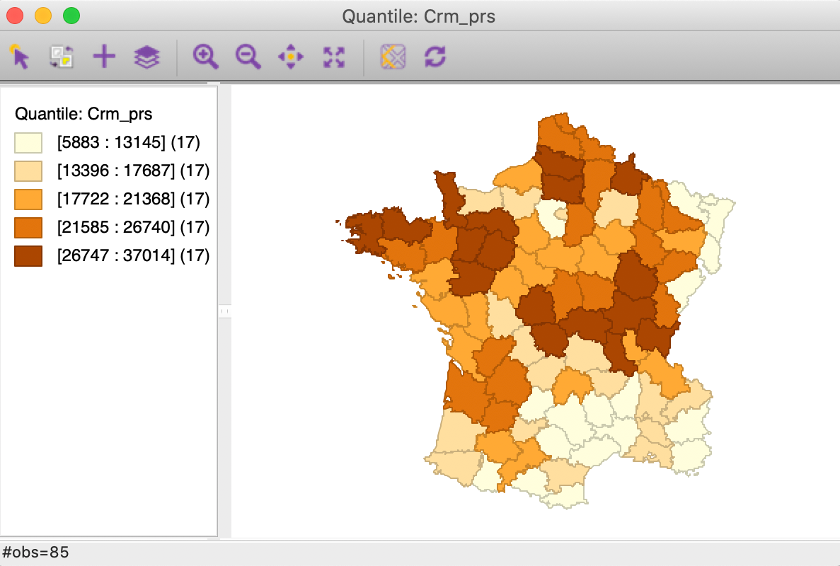
Figure 6: Quintile map - Crime against persons

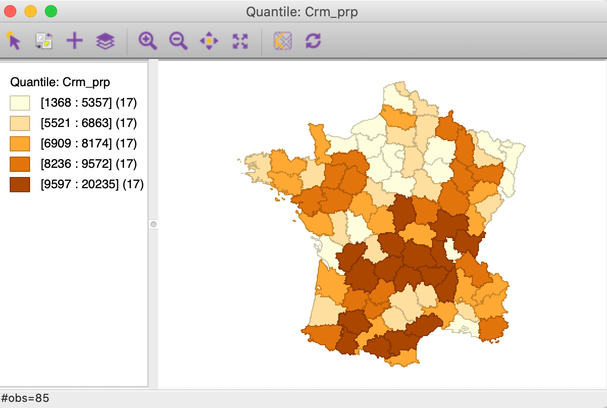
Figure 7: Quintile map - Crime against property

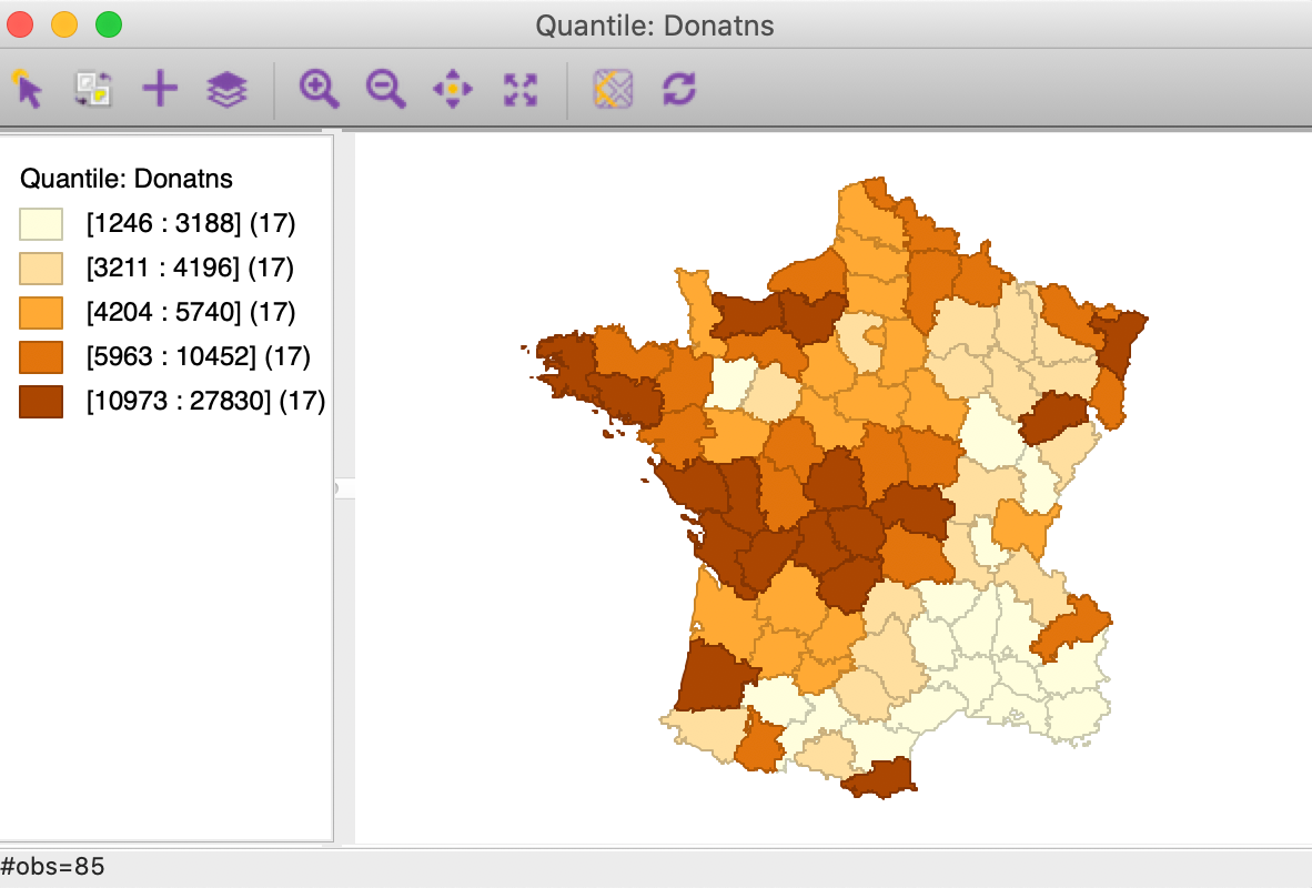
Figure 8: Quintile map - Donations

These maps illustrate the challenge encountered when trying to quantify multivariate spatial correlation, in that they bring out very different patterns. For example, as we may recall from previous Chapters, we notice the concentration of lowest quintile values in the south-east of the country for Donatns (in Figure 8), that is somewhat matched by a similar pattern for Crm_prs (in Figure 6). However, for Crm_prp, the opposite seems to be the case (Figure 7). The lack of correspondence is also indicated by a fairly weak pairwise correlation between these variables: 0.255 between Crm_prs and Crm_prp, 0.134 between Crm_prs and Donatns, and -0.082 between Crm_prp and Donatns (see Anselin 2019, 141).

We further summarize the patterns by means of a Local Geary cluster map for each individual variable, shown in Figures 9 to 11. This confirms the lack of match between the individual spatial distributions (for queen contiguity, with 999 permutations and p=0.05). We find confirmation of the strong Low-Low cluster in the south-east for Crm_prs and Donatns, but for Crm_prp, there seems to be a small Low-Low cluster in the north. Also note several instances of spatial outliers, as well as one example where positive spatial autocorrelation could not be classified for Crm_prp (i.e., Other Positive, in Figure 10).

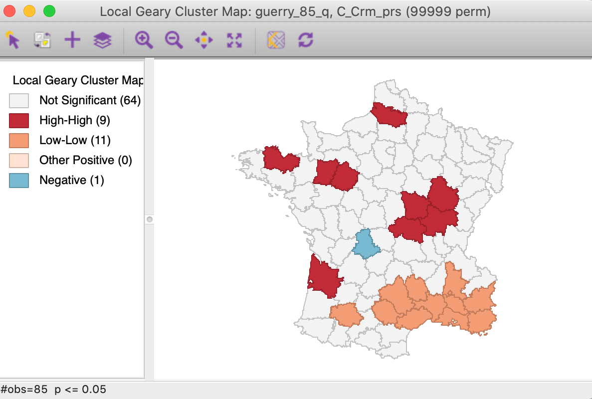
Figure 9: Local Geary cluster map - Crime against persons

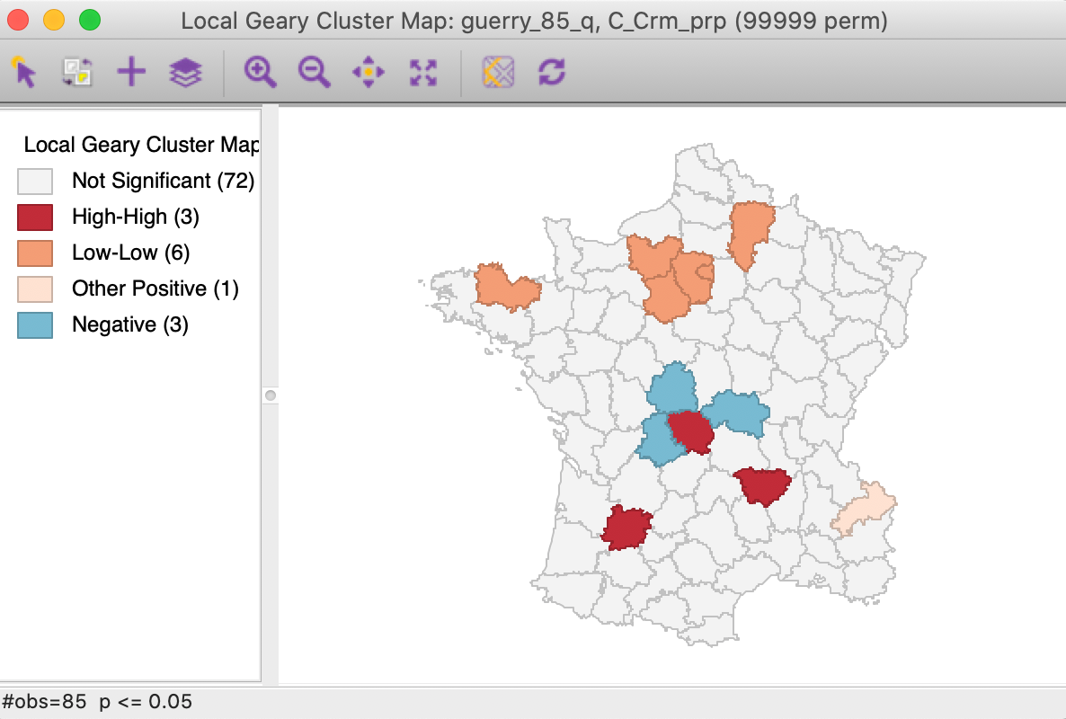
Figure 10: Local Geary cluster map - Crime against property

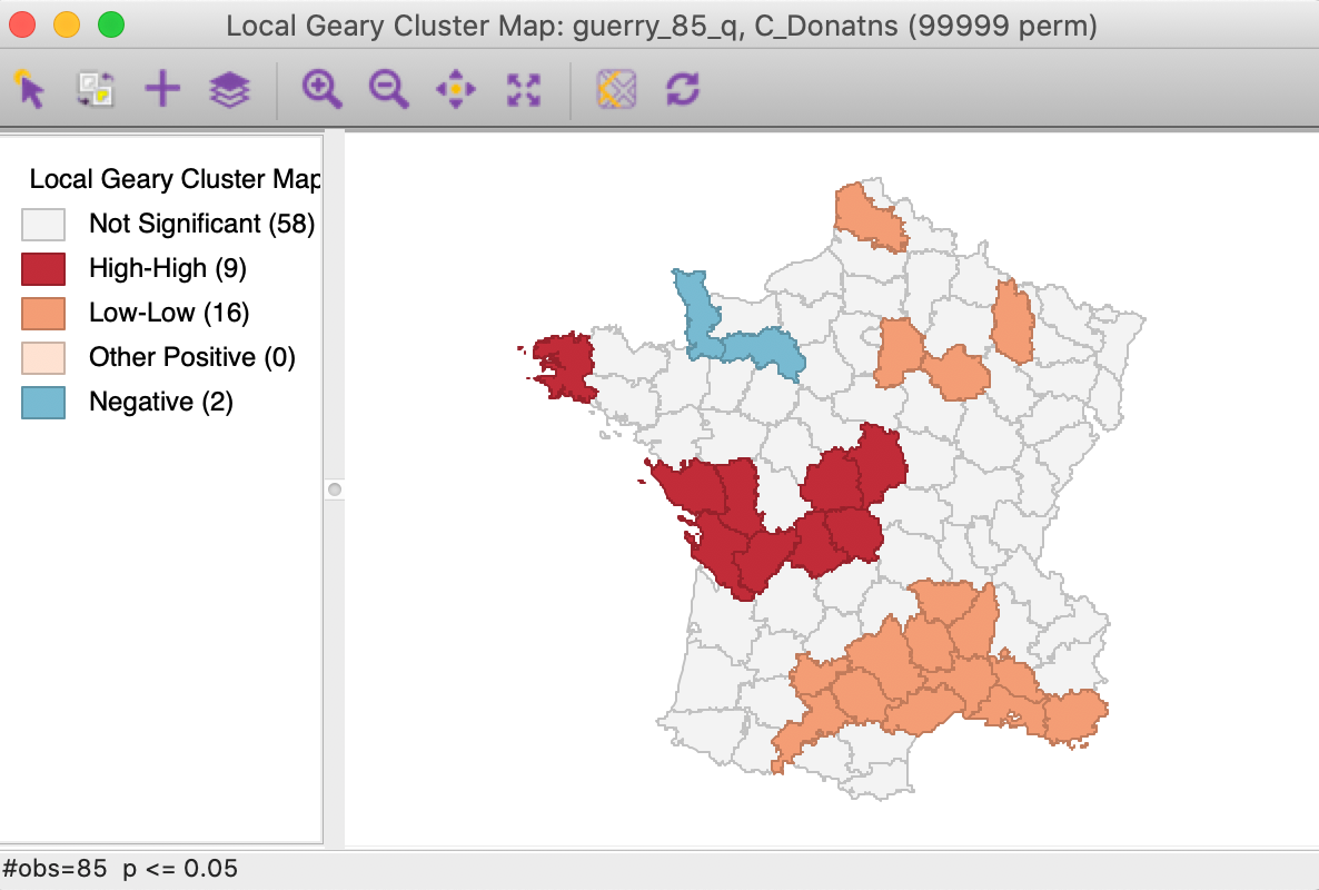
Figure 11: Local Geary cluster map - Donations

A final summary is provided by the co-location map in Figure 12.³ This shows the degree of overlap (or, rather, lack thereof) between the significant locations (at p=0.05) for each of the three Local Geary analyses. Only one observation is significant for all three variables, but it is a spatial outlier for Crm_prs and Crm_prp and part of a High-High cluster for Donatns, suggesting conflicting patterns. The map also shows that 39 observations are not significant for all three variables (0 in the legend), whereas 45 indicate a conflict (significant for one or two, but not three of the variables).

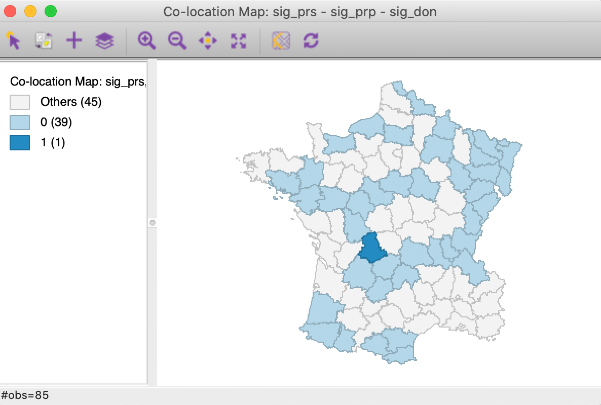
Figure 12: Colocation map - significant locations

In sum, this example highlights the complexity of trying to draw a conclusion about a multivariate spatial correlation pattern from the univariate analysis of the constituent variables.

Multivariate analysis

The Multivariate Local Geary functionality is invoked from the fourth group in the Cluster Maps toolbar icon drop down list (see Figure 1), or from the menu as Space > Multivariate Local Geary.

The variable selection dialog allows for multiple variables to be chosen. In our example, we continue with Crm_prs, Crm_prp and Donatns, with the spatial weights set to guerry_85_q, as in Figure 13.

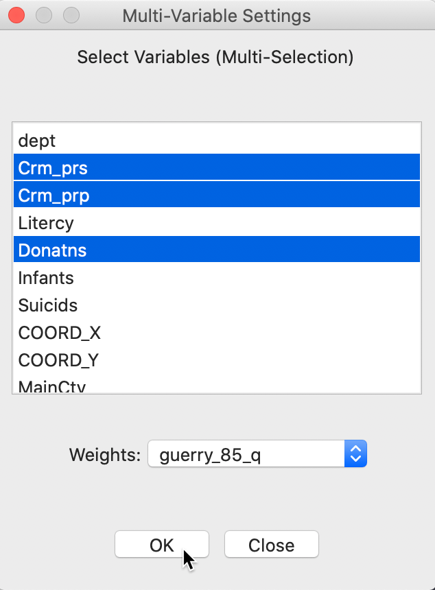
Figure 13: Multivariate local Geary variable selection

As before, a dialog offers the option of a significance map and a cluster map, with the latter as the default. To illustrate the two types of results, we check both options.

With all the other options set to their defaults (999 permutations, p = 0.05), this yields the significance and cluster maps shown in Figure 14.

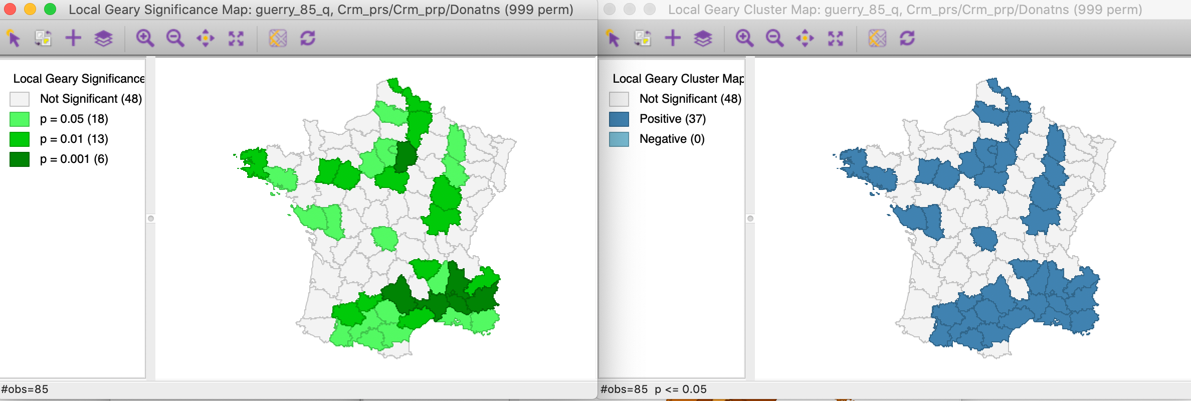
Figure 14: Multivariate local Geary significance and cluster map

Note that for this p-value, we obtain 37 positive clusters, but the single location we identified in Figure 12 is not one of them. The location of the observations with the highest significance in the south-east suggests that the similarity between Crm_prs and Donatns may overwhelm the effect of the third variable. Since the Multivariate Local Geary is a sum of the individual Local Geary, two very small (positive spatial autocorrelation) squared distances may compensate for a larger third one and yield significance in a multivariate world.

All the usual options regarding the number of permutations, the significance filter, and saving the results hold as for any other local spatial statistic in GeoDa. While we do not pursue this further here, it should be noted that a sensitivity analysis with respect to different significance levels is highly recommended.

Interpretation

The results of the Multivariate Local Geary significance or cluster map are not always easy to interpret. Mainly, this is because we tend to simply superimpose the results of the univariate tests, whereas the multivariate statistic involves different tradeoffs.

As mentioned, the problem of multiple comparisons means that the use of the default p-value of 0.05 is almost certainly misleading. A useful alternative is to use the False Discovery Rate, although this only works in small to medium sized data set, due to the maximum on the number permutations in the current implementation of GeoDa. In our example, a p-value of 0.01 also corresponds roughly to the FDR. We illustrate the effect of tightening the p-value in Figure 15 (we increased the number of permuations to 99,999, but no observations were significant at p < 0.001). The number of significant locations in cut in half and reduced to 18. The strongest cluster is found in the south-east.

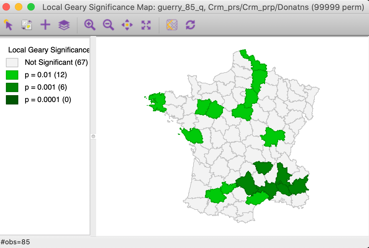
Figure 15: Multivariate local Geary significance map - p = 0.01

Multivariate clusters and 3D scatter plot

In order to illustrate the complexity of the multivariate case, Figure 16 shows three neighboring highly significant locations in the cluster selected in both the significance map and a 3D data cube. The links to the neighbors are also highlighted. This shows that even though the observations in question are very close in multi-attribute space, some of their neighbors are much further removed. This highlights the tradeoffs involved in the averaging of the individual squared distances from the Local Geary statistics. This is not always intuitive. With three variables, this can be visualized in a 3D data cube, but with more variables, this is much harder.

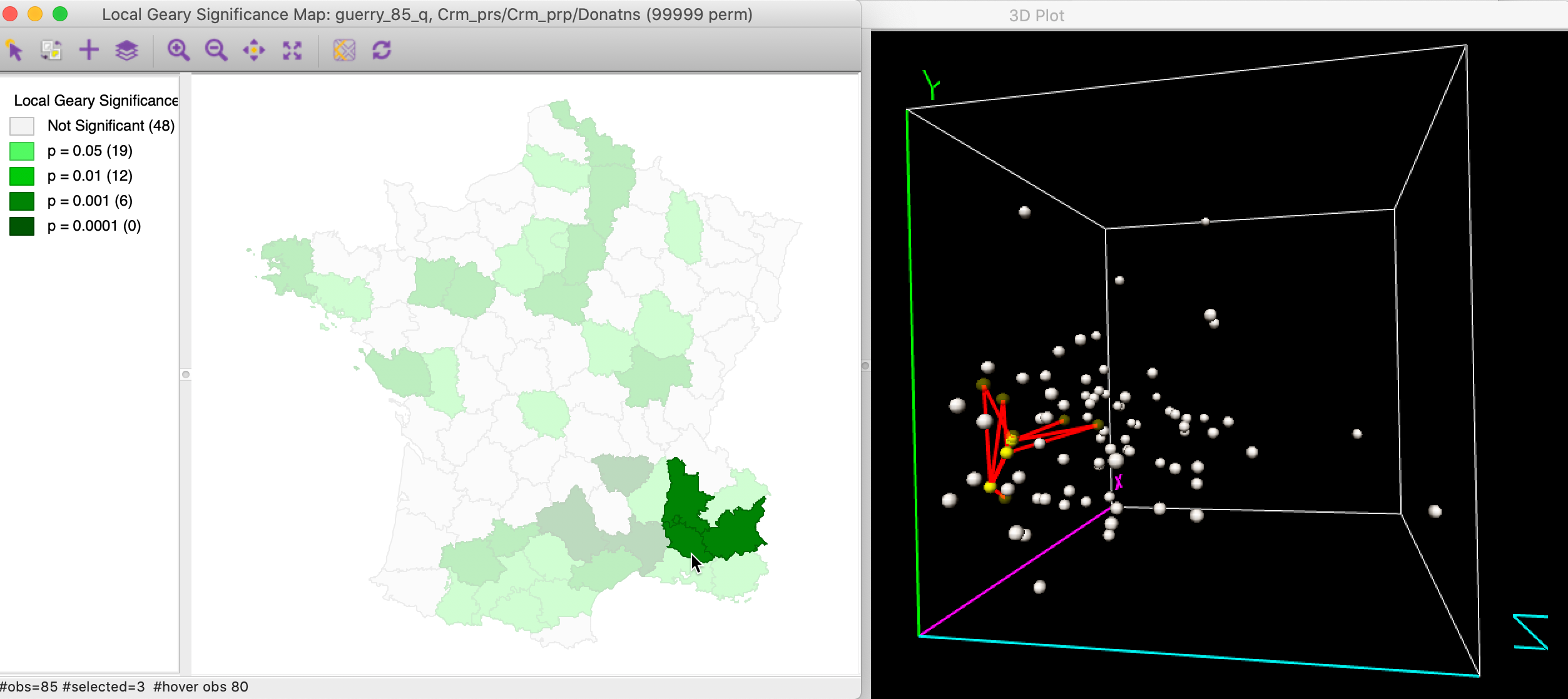
Figure 16: Multivariate local cluster in 3D data cube

Multivariate clusters and PCP

We pursue this further with an example that uses six variables: Crm_prs, Crm_prp, Litercy, Donatns, Infants and Suicids, again with queen contiguity. The significance map, for 99,999 permutations and with p=0.01 is shown in the left panel of Figure 17. Two highly significant locations are selected and their corresponding paths in a parallel coordinate plot highlighted in the right panel. In this example, the neighbors track each other almost perfectly on all six dimensions.

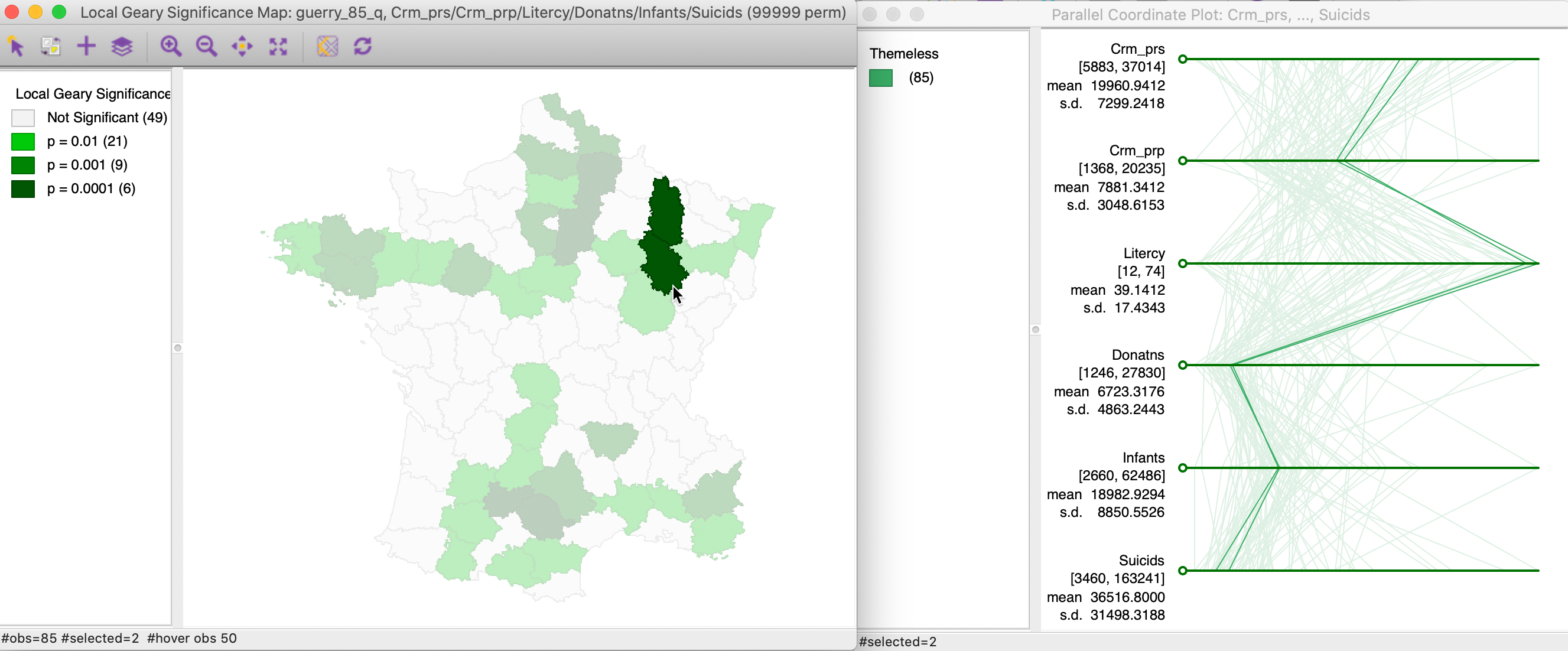
Figure 17: Multivariate local cluster and PCP (1)

Figure 18 shows an example where the intuition is much less clear. Two other highly significant neighboring locations are selected in the left-hand panel, and their corresponding paths shown on the right. In this instance, while the distances between the paths are small, there is much less of a close match.

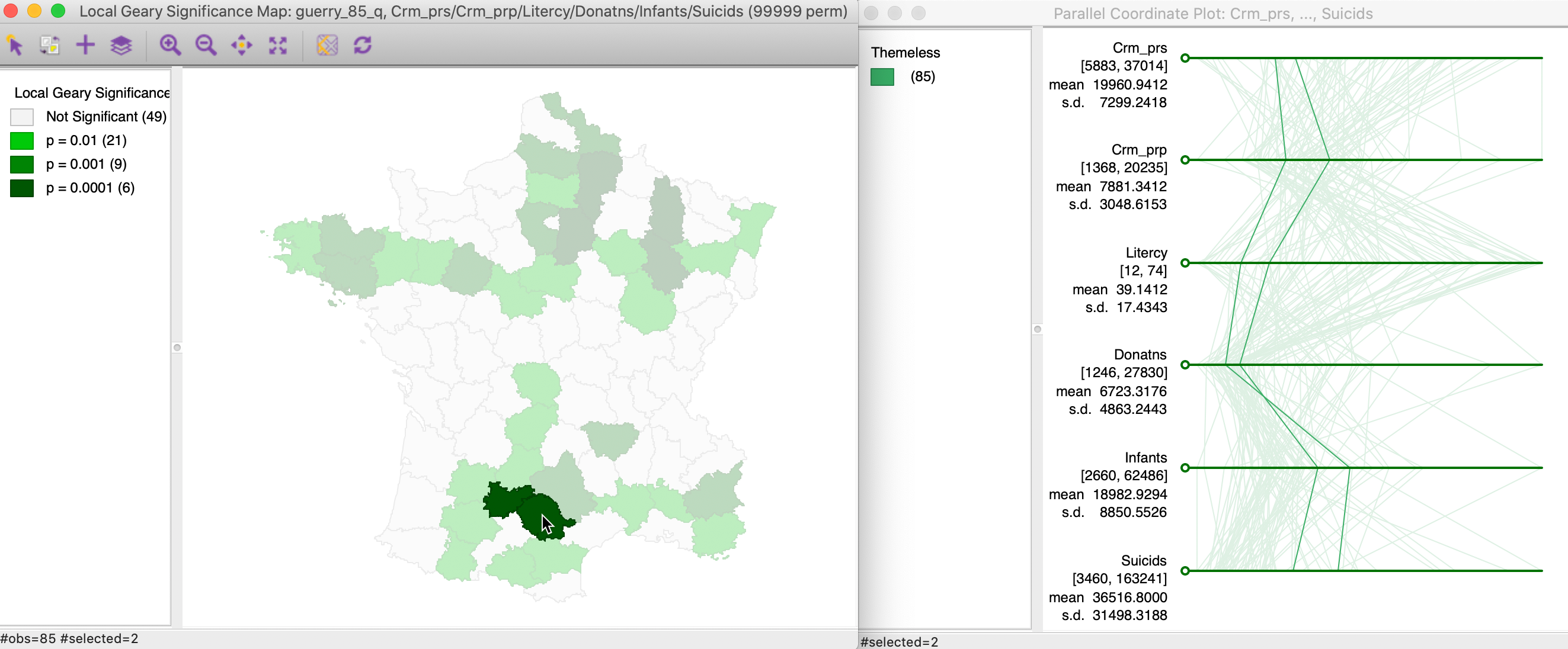
Figure 18: Multivariate local cluster and PCP (2)

Nevertheless, this illustrates how a judicious use of multiple graphs and maps can create insight into the complex tradeoffs between attribute similarity in a higher dimension for neighboring locations.

Local Neighbor Match Test

Principle

An alternative approach to visualize and quantify the tradeoff between geographical and attribute similarity was suggested by Anselin and Li (2020) in the form of what is called a local neighbor match test. The basic idea is to assess the extent of overlap between k-nearest neighbors in geographical space and k-nearest neighbors in multi-attribute space.

In GeoDa, this is a simple intersection operation between two k-nearest neighbor weights matrices, one computed for the variables (standardized) and one using geographical distance. We can then quantify the probability that an overlap occurs between the two neighbor sets. This corresponds to the probability of drawing \(v\) common neighbors from the \(k\) out of \(n - 1 - k\) possible choices as neighbors, a straightforward combinatorial calculation.

More formally, the probability of \(v\) shared neighbors out of \(k\) is: \[p = C(k,v).C(N-k,k-v) / C(N,k),\] where \(N = n - 1\) (one less than the number of observations), \(k\) is the number of nearest neighbors considered in the connectivity graphs, \(v\) is the number of neighbors in common, and \(C\) is the combinatorial operator. Alternatively, a pseudo p-value can be computed based on a permutation approach, although that is not pursued in GeoDa.

The degree of overlap can be visualized by means of a cardinality map (a special case of a unique values map), where each location indicates how many neighbors the two weights matrices have in common. In addition, different p-value cut-offs can be employed to select the significant locations, i.e., where the probability of a given number of common neighbors falls below the chosen p.

In practice, the value of \(k\) may need to be adjusted (increased) in order to find meaningful results. In addition, the k-nearest neighbor calculation becomes increasingly difficult to implement in very high attribute dimensions, due to the empty space problem.

The idea of matching neighbors can be extended to distances among variables obtained from dimension reduction techniques, such as multidimensional scaling, covered in a later Chapter (see also the more detailed discussion in Anselin and Li 2020).

In contrast to the approach taken for the Multivariate Local Geary, the local neighbor match test focuses on the distances directly, rather than converting them into a weighted average. Both measures have in common that they focus on squared distances in attribute space, rather than a cross-product as in the Moran statistics.

Implementation

We illustrate the local neighbor match test by means of the Guerry data set. We use the same six variables as before: Crm_prs, Crm_prp, Litercy, Donatns, Infants and Suicids. We first illustrate the logic behind the method and then show its implementation in GeoDa.

We start by creating two k-nearest neighbor weights matrices for k=6, one based on Euclidean geographical distance, the other on multi-variable distance using the six specified variables in z-standardized form. Both matrices should be contained in the Weights Manager.

Intersection between connectivity graphs

We compare the connectivity graphs for the geographical (guerry_85_kd6) and the multi-variable (guerry_85_k6v) weights. They are shown side-by-side in Figure 19, with the geographical connectivity on the left. Whereas the latter has the familiar form, the multi-variable connectivity is quite complex and shows connections between locations that are far apart in geographical space.

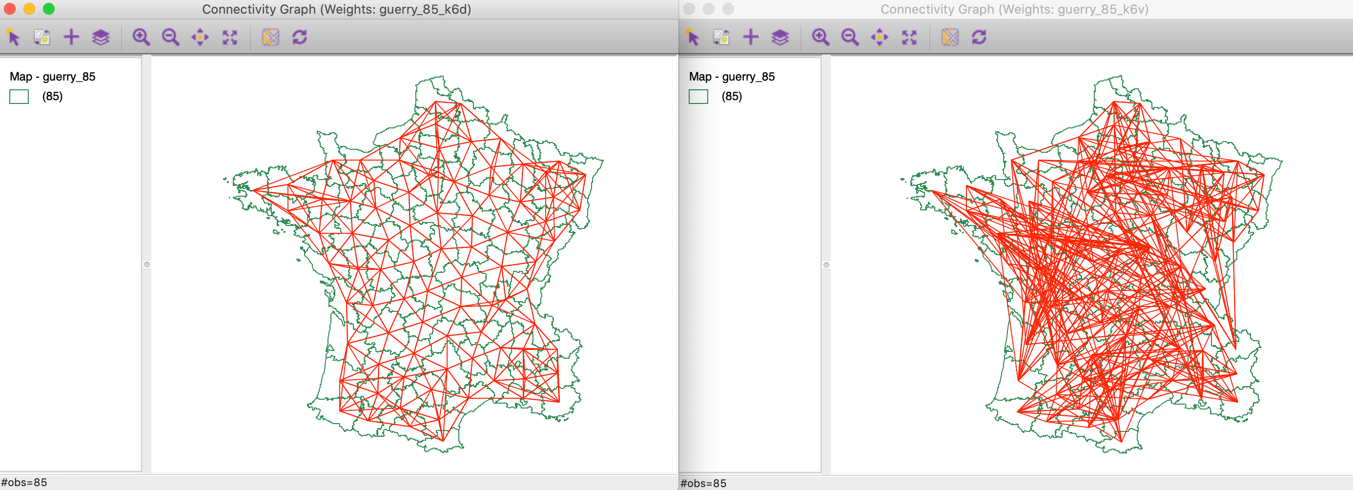
Figure 19: Connectivity graph for distance k=6 and multivariable k=6

In the Weights Manager, we select the Intersection button for these two weights to create a new gal file. The connectivity graph for the common neighbors is shown in Figure 20. This illustrates the logic underlying the local neigbhor match test. What remains to be done is to assess the extent to which the number of coincident neighbors is due to chance, or unlikely under random matching.

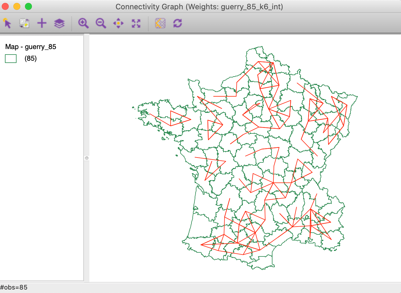
Figure 20: Intersection between connectivity graphs

Testing the local neighbor match

We invoke the local neighbor match test as the last item in the Cluster Maps toolbar icon, as show in Figure 1, or from the menu as Space > Local Neighbor Match Test. Next follows a query for the variables, in the usual dialog, shown in Figure 21. We select the same six variables as before. In addition, we set the Number of Neighbors to 6, and use Euclidean Distance for both neighbor criteria. Finally, we also make sure that the variables are used in standardized form.

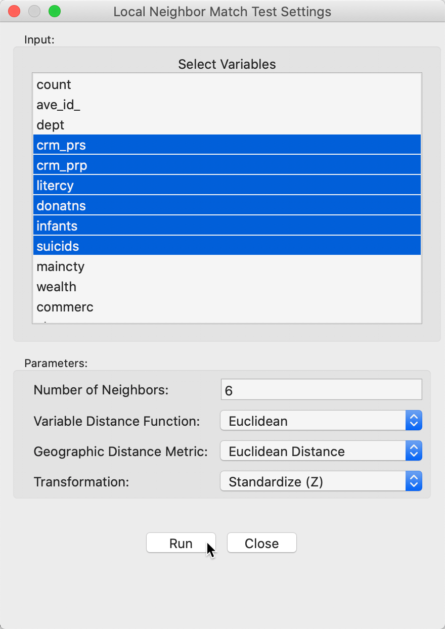
Figure 21: Local neighbor match variable selection

After starting the procedure, a simple dialog in Figure 22 appears, in order to specify whether to save the common neighbor cardinality and associated p-value in the table. This must be done in order to refer back to the probability for later visualization.

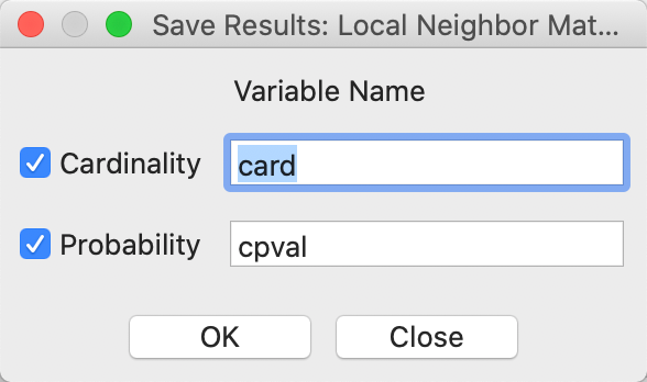
Figure 22: Local neighbor match save results

The result of the analysis is a special unique values map that shows the cardinality (the number) of common neighbors for each location, as well as the corresponding links from the connectivity graph, as in Figure 23. This is essentially the same graph as in Figure 20, but with the cardinality added as a shade (darker shade for more neighbors). The commonality ranges from 1 location with 5 neighbors, and 4 with 4, to 25 with one neighbor.

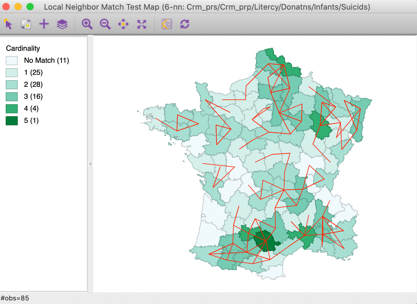
Figure 23: Local neighbor match connectivity cardinality

In addition, the cardinality and associated probability are added to the data table, as in Figure 24.

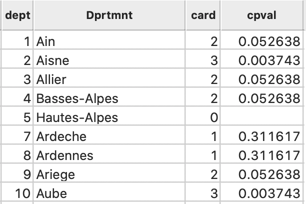
Figure 24: Local neighbor match cardinality and p-value

Significance

As such, the neighbor cardinality map does not indicate any significance. It is clear that having 5 neighbors out of 6 is fairly rare (in fact, its probability is 0.000001), but it is not clear where to draw the line between significant and not. We can now use the Selection Tool in the table to select all observations with a p-value of less than 0.05 (or any other relevant value). This results in the significant locations being highlighted in the cardinality map, as in Figure 25. It turns out that for this cut-off, there are 21 significant observations, all with 3 or more neighbors in common.

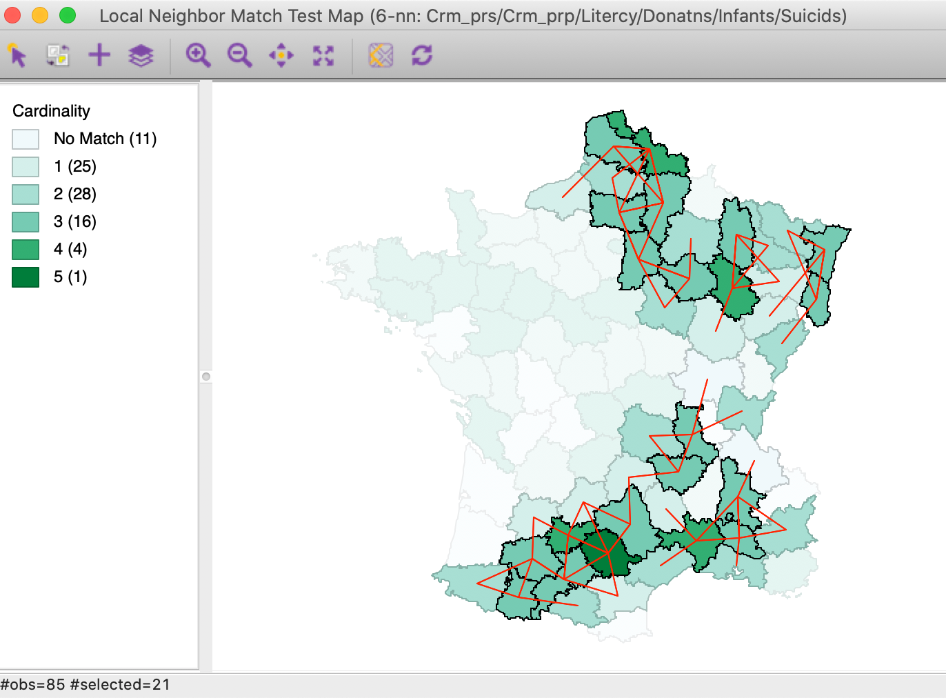
Figure 25: Local neighbor match significant locations (p=0.05)

We can further decompose the connectivity structure for the significant locations by highlighting them in both original connectivity graphs, as in Figure 26.⁴ In the subset of significant locations in the south-west corner of the country, we notice a remarkable match between the two connectivity structures. In contrast, some of the significant locations in the north have multi-attribute connections with locations that are geographically far removed.

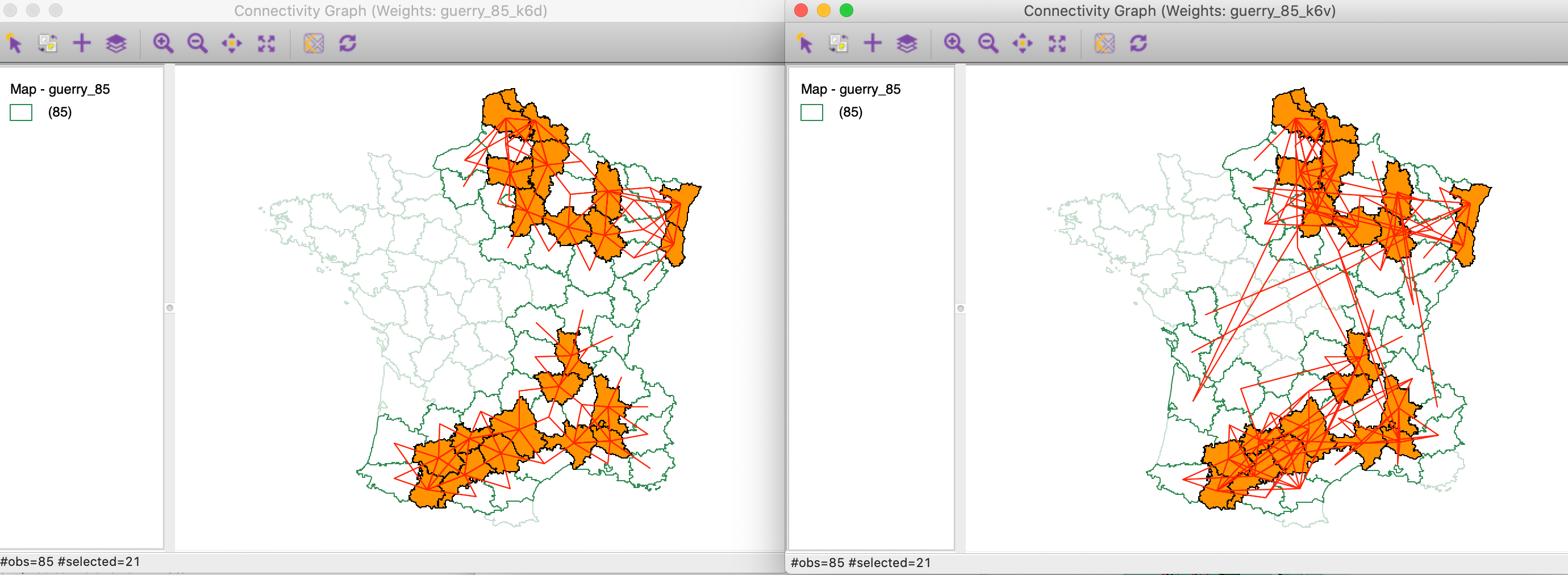
Figure 26: Local neighbor match significant locations in connectivity graphs

Local neighbor match and Multivariate Local Geary

To close, we compare the most significant locations identified by the Multivariate Local Geary and the local neighbor match test. We used 99,999 permutations and a p-value of 0.01 for the Local Geary cluster map.

In Figure 27 we select the most significant location in the local neighbor match test map on the left. Its 5 neighbors that are common on the two criteria are highlighted as well. In the cluster map on the left, we find the corresponding location and its neighbors. As it turns out, the central location (department of Tarn) is identified as having a p-value of 0.0001 in the cluster map. One of its neighbors achieves the same value, while two have p=0.001, and on p = 0.01. However, one of the common neighbors is not significant according to the Multivariate Local Geary. Nevertheless, the match between the two approaches is striking, confirming that both use a similar perspective.

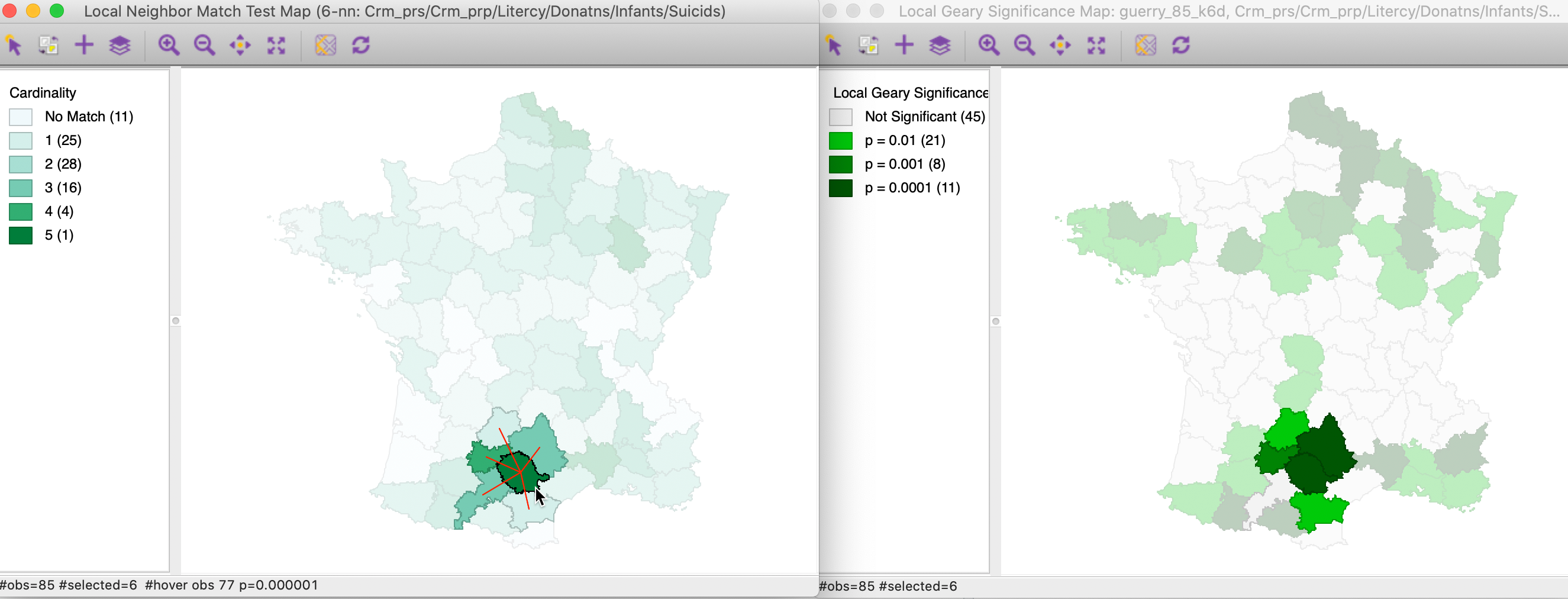
Figure 27: Local neighbor match significant locations and Multivariate Local Geary (1)

In Figure 28, we take the opposite approach. We select the 11 locations in the right-hand map that are significant at p=0.0001. The left-hand panel shows the matching selection in the local neighbor match test. In addition to the Tarn department with 5 matches, we also find three of the four departments with 4 matches to be identified in both maps. In all, of the 11 significant Local Geary locations, 9 are significant at p=0.05 in the local neigbhor match map. Interestingly, two significant Local Geary locations (Basses-Alpes and Ariege) only have two common neighbors.

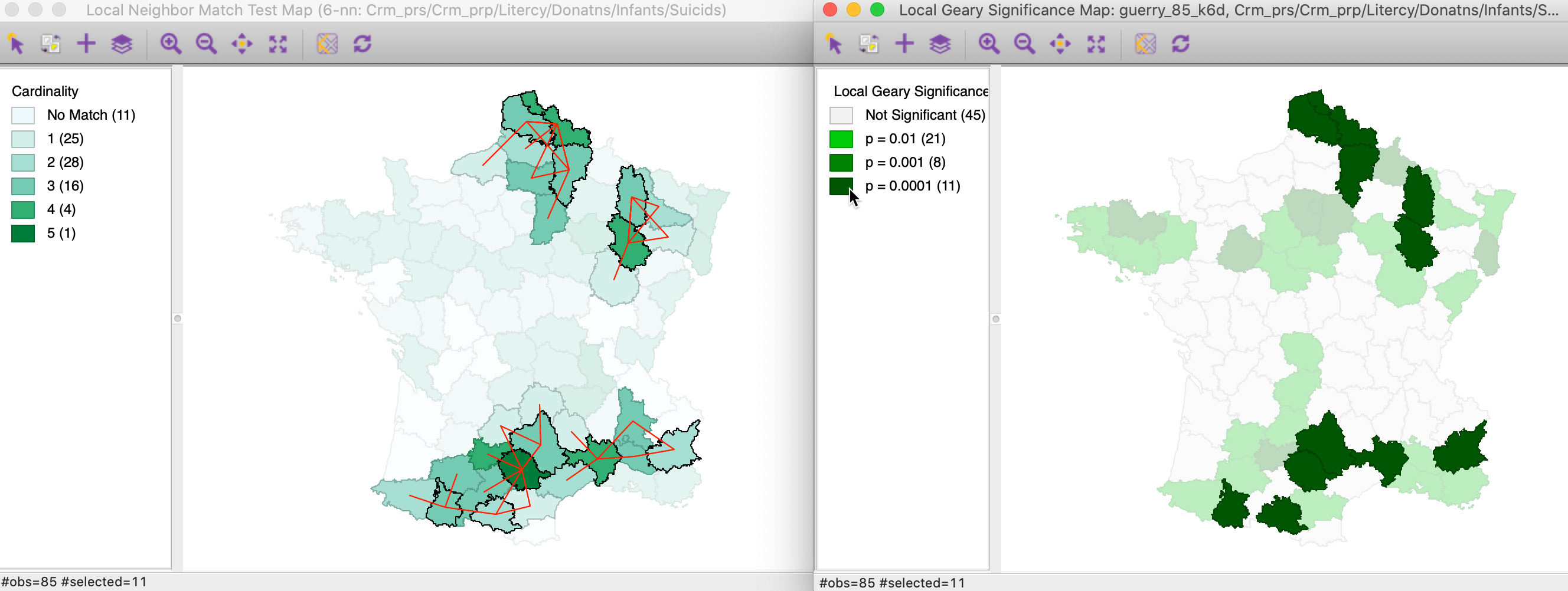
Figure 28: Local neighbor match significant locations and Multivariate Local Geary (2)

We investigate the connectivity pattern for those two locations more closely in Figure 29. In the right-hand panel, we see how the multi-attribute neighbors for both departments tend to be far removed geographically. In the averaging operation that is behind the Multivariate Local Geary, the difference with the contiguous locations are averaged out. In the local neighbor match test, the focus is singularly on the distances themselves.

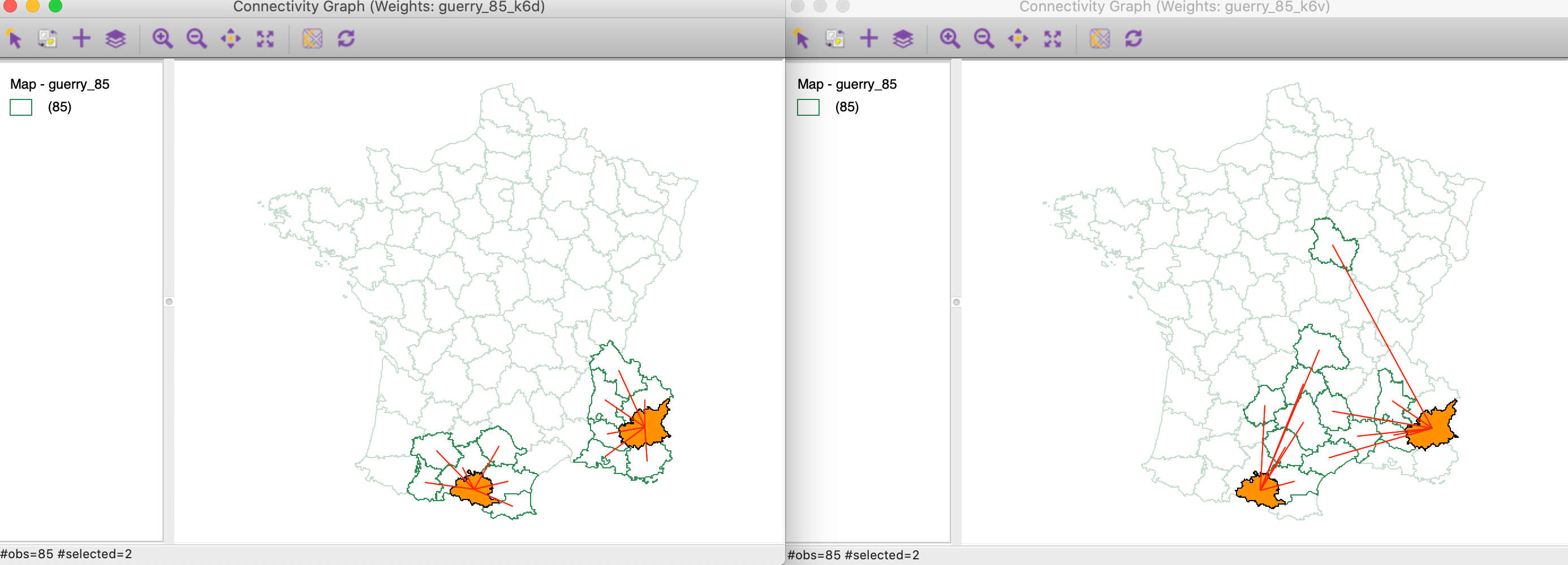
Figure 29: Significant Multivariate Local Geary locations with only two matching neighbors

In spite of these slight discrepancies between the two methods, they tend to identify the same broad clusters. Given that it has fewer issues with determining the proper p-value, the local neighbor match test thus provides a viable alternative to detect multivariate spatial clusters.

References

Anselin, Luc. 2019. “A Local Indicator of Multivariate Spatial Association, Extending Geary’s c.” Geographical Analysis 51 (2): 133–50.

Anselin, Luc, and Xun Li. 2020. “Tobler’s Law in a Multivariate World.” Geographical Analysis 52 (4): 494–510. https://doi.org/10.111/gean.12237.

Anselin, Luc, Ibnu Syabri, and Oleg Smirnov. 2002. “Visualizing Multivariate Spatial Correlation with Dynamically Linked Windows.” In New Tools for Spatial Data Analysis: Proceedings of the Specialist Meeting, edited by Luc Anselin and Sergio Rey. University of California, Santa Barbara: Center for Spatially Integrated Social Science (CSISS).

Dray, Stéphane, Sonia Saïd, and François Débias. 2008. “Spatial Ordination of Vegetation Data Using a Generalization of Wartenberg’s Multivariate Spatial Correlation.” Journal of Vegetation Science 19: 45–56.

Fotheringham, A. Stewart, Chris Brunsdon, and Martin Charlton. 2002. Geographically Weighted Regression. Chichester: John Wiley.

Lee, Sang-Il. 2001. “Developing a Bivariate Spatial Association Measure: An Integration of Pearson’s r and Moran’s I.” Journal of Geographical Systems 3: 369–85.

Lin, Jie. 2020. “A Local Model for Multivariate Analysis: Extending Wartenberg’s Multivariate Spatial Correlation.” Geographical Analysis 52 (2): 190–210.

Wartenberg, Daniel. 1985. “Multivariate Spatial Correlation: A Method for Exploratory Geographical Analysis.” Geographical Analysis 17: 263–83.

---

1. University of Chicago, Center for Spatial Data Science – anselin@uchicago.edu↩︎

2. See Anselin (2019) for further technical discussion.↩︎

3. This map is constructed by first turning the significant locations in each significance map into an indicator variable for the selection (Save Selection), and then using these three variables in a co-location map.↩︎

4. The fill color of selected has been changed to orange to bring the selected locations out more clearly.↩︎

GeoDa is maintained by lixun910. This page was generated by GitHub Pages using the Cayman theme by Jason Long.