Local Spatial Autocorrelation (4)

LISA for Discrete Variables

Introduction

So far, we have considered the application of local spatial autocorrelation statistics to continuous variables. In this Chapter, we move to discrete variables, and, more specifically, binary variables. We cover the application of the LISA principle to this case in the form of a univariate local join count statistic and extend this to a multivariate setting as well. In the latter, we need to make a distinction between situations where the two discrete variables can co-occur (i.e., take the value of 1 for the same location), and where they cannot.

We close with a discussion of the notion of a Quantile LISA as a special case of the local join count.

To illustrate these statistics, we use two data sets that deal with the 77 community areas in Chicago, the sample data sets Chicago commpop and Chicago Health.

Objectives

• Identify clusters in binary variables by means of the local join count statistic

• Distinguish between co-location and no co-location in a bivariate binary variable case

• Identify multivariate co-location clusters in binary variables with the local join count statistic

• Apply the Quantile LISA concept to simplify the assessment of univariate and multivariate clusters

GeoDa functions covered

• Space > Univariate Local Join Count
• Space > Bivariate Local Join Count
• Space > Co-location Join Count
• Space > Univariate Quantile LISA
• Space > Multivariate Quantile LISA

Preliminaries

We use two data sets from the GeoDa Center data set collection that contain information on the 77 Community Areas in Chicago.

• Chicago commpop: Chicago community area population and percent change for 2000 and 2010

• Chicago Health: Chicago community area health and socio-economic indicators

After downloading these data sets, we will also need to construct a spatial weights matrix, such as queen contiguity.²

Univariate Local Join Count Statistic

Principle

For binary variables, coded as 0 and 1, the global spatial autocorrelation statistic of choice is the join-count statistic (see Cliff and Ord 1973). This statistic consists of counting the joins that correspond to occurrences of value pairs at neighboring locations. The three cases are joins of \(1-1\) (so-called BB joins, for black-black), \(0-0\) (so-called WW joins, for white-white), and \(0-1\) (so-called BW joins). The former two are indicators of positive spatial autocorrelation, the latter of negative spatial autocorrelation.

Our interest lies in identifying co-occurrences of uncommon events, i.e., situations where observations that take on the value of 1 constitute much less than half of the sample (the definition of what is 1 or 0 can easily be reversed to make sure this condition is met). We therefore focus on the BB join counts. While this is not an absolute requirement, the way the inference is obtained requires that the probability of obtaining a large number of like neighbors is small, hence a basis for rejecting the null hypothesis. When the proportion of observations with 1 is larger than half, then the probability of a small number of neighbors will be small, which is counter our logic.³

With the variable \(x_i\) at location \(i\) taking either the value of 1 or 0, a global BB join count statistic can be written as: \[BB = \sum_i \sum_j w_{ij} x_i x_j,\] where \(w_{ij}\) are the elements of a binary spatial weights matrix. In other words, a join is counted when \(w_{ij} = x_i = x_j = 1\). In all other instances, either when there is a mismatch in \(x\) between \(i\) and \(j\), or a lack of a neighbor relation (\(w_{ij} = 0\)), the term on the right-hand side does not contribute to the double sum.

Following the logic in Anselin (1995), Anselin and Li (2019) recently introduced a local version of the BB join count statistic as: \[BB_i = x_i \sum_j w_{ij}x_j,\] where \(x_{i,j}\) can only take on the values of 1 and 0, and, again, \(w_{ij}\) are the elements of a binary spatial weights matrix (i.e., not row-standardized).

The statistic is only meaningful for those observations where \(x_i = 1\), since for \(x_i = 0\) the result will always equal zero. When \(x_i = 1\), it corresponds to the sum of neighbors for which the value \(x_j = 1\). In this sense, it is similar in spirit to to the local second order analysis for point patterns outlined in Getis (1984) and Getis and Franklin (1987), where the number of points are counted within a given distance \(d\) of an observed point. The distance cut-off \(d\) could readily form the basis for the construction of the spatial weights \(w_{ij}\), which yields the join count statistic as a count of events (points) within the critical distance from a given point (\(x_i = 1\)).

The main difference between the two concepts is the underlying data structure: in the point pattern perspective, the locations themselves are considered to be random, whereas the local join count statistic is based on a lattice perspective. The latter considers a finite set of known locations, for which both events (\(x_i = 1\)) and non-events (\(x_i = 0\)) are observed. In point patterns analysis, one does not know the locations where events might have happened, but did not.

In addition, the local join count statistic also has the same structure as the numerator in local \(G_i\) statistic of Getis and Ord (1992), when applied to binary observations (and with a binary weights matrix). The numerator in this statistics is \(\sum_j w_{ij} x_j\), which is identical to the multiplier in the local join count statistic. However, the difference between the two statistics is that the local G counts the neighbors with \(x_j = 1\) for all locations, including the ones where \(x_i = 0\). Such observations are ignored in the computation of the local join count statistic as outlined above. In a sense, the local join count statistic could thus be considered a constrained form of the local G statistic, limited to observations where \(x_i = 1\).

Inference can be based on a hypergeometric distribution, or, as before, on a permutation approach. Given a total number of events in the sample of \(n\) observations as \(P\), we consider the number of neighbors of location \(i\) for which \(x_i = 1\), i.e., conditional upon observing 1 at this location. The number of neighbors with \(x_j = 1\) is represented by \(p_i\). The probability of observing exactly \(p_i = p\), conditional upon \(x_i = 1\) follows the hypergeometric distribution for \(n - 1\) data points and \(P - 1\) events: \[\mbox{Prob}[p_i = p | x_i = 1] = \frac{ {{P-1} \choose {p}} { {N - P - 2} \choose {k_i - p} }}{ { {N-1} \choose {k_i}} },\] where \(k_i\) is the number of neighbors for observation \(i\).

Instead, a conditional permutation procedure can be followed to compute a pseudo \(p\)-value, in the usual fashion. It should be noted that this is not equivalent to the exact probability approach, which actually underestimates uncertainty, because it ignores the uncertainty associated with observing \(x_i =1\).

In practice, the permutation approach is to be preferred, since it does not require any parametric assumptions and is formulated as a classical one-sided hypothesis test against the null hypothesis of spatial randomness. In what follows, we only consider the conditional permutation approach. Further technical details are provided in Anselin and Li (2019).

Implementation

We will illustrate the local join count statistic for the popplus binary variable in the commpop data set. This is a binary variable corresponding to community areas that achieved positive population change between the census years of 2000 and 2010. The unique values map in Figure 1 showns how only 17 out of the 77 community areas show population increase.

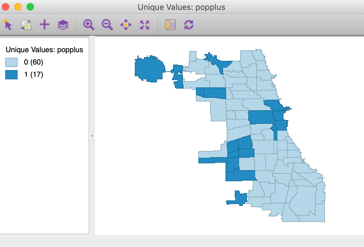
Figure 1: Unique values map for popplus

The univariate local join count statistic is invoked from the third group in the Cluster Maps toolbar icon, as in Figure 2, or, from the menu, as Space > Univariate Local Join Count.

Figure 2: Univariate Local Join Count toolbar icon

After activating this option, a variable selection dialog appears, from which we choose popplus. In addition, we make sure to have a spatial weights matrix listed, here chicago_commpop_q (these weights will be used in non-standardized binary form).

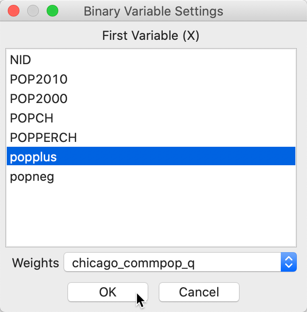
Figure 3: Univariate Local Join Count variable selection

Local significance map

In contrast to the other local statistics, there is only a significance map for the local join count statistic, since all identified locations refer to clusters of a 1, surrounded by more neighbors with 1 than would be the case under spatial randomness. In other words, there is no distinction between high-high and low-low, only the former is a valid concept for a cluster of binary variables.

The result for the default 999 permutations and p=0.05 is shown in Figure 4. As it turns out, only 3 of the 17 locations can be considered the cores of actual clusters (recall that an actual cluster consists of both the observation and its neighbors). In addition, the associated p-values are fairly weak.

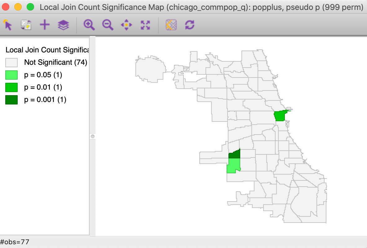
Figure 4: Local significance map for popplus

Cluster identification

In order to assess the actual spatial reach of the clusters, we select the significant locations in the significance map and invoke Connectivity > Show Selection and Neighbors. In Figure 5, the significant cores are shown with a red outline together with their queen contiguity neighbors.

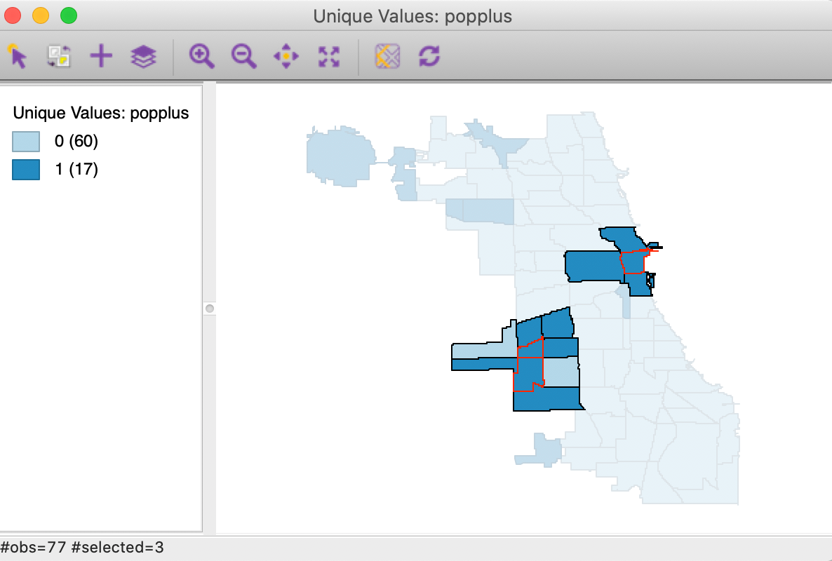
Figure 5: Cluster identification for local join count

Saving the results

An alternative way to check on the neighbor structure of the significant locations is to use the Save Results option. Similar to its operation for the other local spatial autocorrelation statistics, this saves the statistic, i.e., the number of BB joins (default variable name JC), the total number of neighbors (NN), and the pseudo p-value (PP_VAL), as in Figure 6. As usual, the new variables are only permanently added to the Table after a Save command.

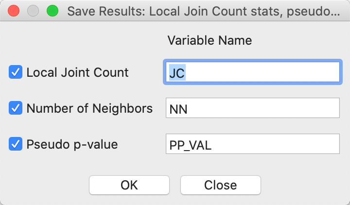
Figure 6: Local Join Count Save Results options

In Figure 7, we show the information for all 17 observations with a value of 1. The three significant locations are West Elsdon, with 5 neighbors out of 6 also taking a value of 1 (yielding a pseudo p-value of 0.001), the Loop, with 3 neighbors out of 3 taking a value of 1 (yielding a pseudo p-value of 0.009), and West Lawn, with 4 neighbors out of 6 taking a value of 1 (yielding a pseudo p-value of 0.013). Note that when none of the neighbors take a value of 1 (i.e., JC=0), GeoDa does not report a p-value. Since this p-value should be the complement of the probabilities associates with all non-zero values for the number of neighbors, it is not meaningful for our inference. Also, observations with a value of \(x_i = 0\) are not considered (i.e., they have no JC statistic or p-value, but the number of neighbors is listed in the table, since that is based on the spatial weights).

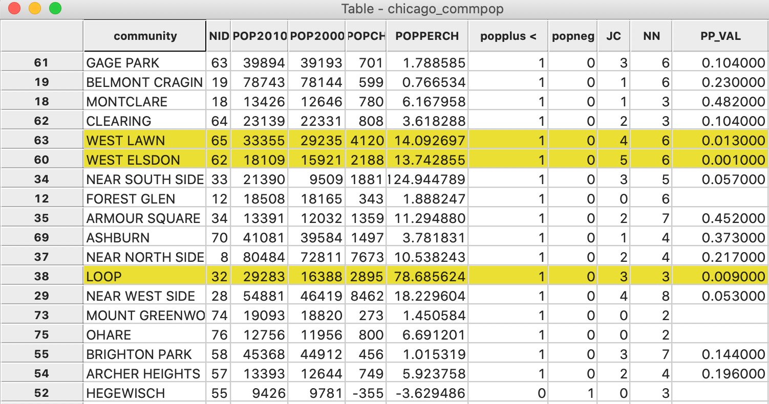
Figure 7: Local Join Count Results in Table

Bivariate Local Join Count Statistic

Principle

In a bivariate binary context, the two variables under consideration, say \(x\) and \(z\), again only take on a value of 0 and 1.

We distinguish between two cases, referred to as co-location and no co-location. In the first, it is possible for both variables to take the same value at a location. In other words, at location \(i\), it is possible to have \(x_i = z_i = 1\). For example, this would be the case when the variables pertain to two different types of events that can occur in all locations, such as the presence of several non-exclusive characteristics (e.g., a city block that is both low-density and commercial, or a parcel that can be single family/multifamily, or owned/rented).

In the no co-location case, whenever \(x_i = 1\), then \(z_i = 0\) and vice versa. In other words, the two events cannot happen in the same location. This would be case where the classification of a location is exclusive, i.e., if a location is of one type, it cannot be of another type (e.g., a zoning classification, or a case-control design). A special case of this design is to assess potential negative spatial autocorrelation, e.g., between the community areas that have positive and those that have negative population change.

Here again, it is important to make sure that the second variable, z, is a rare occurrence, appearing in less than half of the sample.

We consider the no co-location situation first. In GeoDa, this is referred to as bivariate local join count, since this is the only setting in which it is operational (the no co-location setup does not work for more than two variables).

In its general form, the expression for a bivariate local join count statistic given in Anselin and Li (2019) is: \[BJC_i = x_i (1 - z_i) \sum_j w_{ij} z_j (1 - x_j),\] with \(w_{ij}\) as unstandardized (binary) spatial weights.

The roles of \(x\) and \(z\) may be reversed, but the statistic is not symmetric, so that the results will tend to differ whether \(x\) or \(z\) is the focus. In addition, it is important to keep in mind that the statistic will only be meaningful when the proportion of the second variable (for the neighbors) in the population is small.

Since the condition of no co-location ensures that \(1 - z_i = 0\) whenever \(x_i = 1\), and vice versa, the statistic simplifies to: \[BJC_i = x_i \sum_j w_{ij} z_j,\] whenever \(x_i = 1\), which are the only locations we are interested in.

Inference can be based on a hypergeometric distribution, considering \(P\) observations with \(x_i = 1\) and \(Q\) observations with \(z_j = 1\). Again, a more robust alternative is based on a permutation approach.

A pseudo p-value can be obtained from a one-sided conditional permutation test. This is implemented by carrying out a series of \(k_i\) draws (with \(k_i\) as the number of neighbors for \(i\)) for each location \(i\) where \(x_i = 1\) (and thus \(z_i = 0\)). The draws are without replacement from n − 1 data tuples \((x_j, z_j)\) of which \(Q\) observations have \(z = 1\) (since \(z_i = 0\)) and \(P − 1\) observations have \(x = 1\). In practice, we only need to draw the \(z_j\), since the matching \(x_j\) in the tuple are zero by construction. The number of times the resulting local join count statistic equals or exceeds the observed value yields a pseudo p-value, in the usual way.

Implementation

To illustrate this statistic, we continue with the commpop example. We are interested in instances of negative spatial autocorrelation, where locations with popneg = 1 are surrounded by more locations with popplus = 1 than would be expected under randomness.

Note that it is important to formulate the research question in this fashion. Since the majority of locations has popneg = 1 (60/77, or 0.78), the phenomenon of a popplus = 1 to be surrounded by locations with popneg = 1 is not rare. In such a situation, the significance test is not meaningful.⁴ This will generally be the case when a variable has more than 50% of the observations equal to 1.

Since only 0.22 of the observations have popplus = 1, we have already considered the extent to which these cluster among themselves by means of a Univariate Local Join Count test. In addition, we could assess the extent to which they group around locations with negative population change. Those instances of popneg = 1 could then be characterized as spatial outliers, i.e., areas with population decline surrounded by neighbors with population increase.

This example is primarily to illustrate the functionality of the bivariate test, and is less of substantive interest.⁵

The Bivariate Local Join Count statistic is invoked from the third group in the Cluster Maps toolbar icon, as shown in Figure 2, or, from the menu, as Space > Bivariate Local Join Count. Next is a dialog from which we select the two binary variables. The first one (\(x\)) is selected from the left-hand column in the dialog, the second (\(z\)) from the right-hand column. In our example, these are popneg and popplus, as shown in Figure 8.

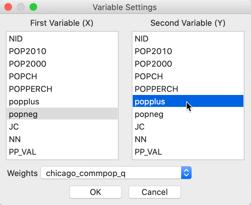
Figure 8: Bivariate local Join Count variable selection

As is the case for the Univariate Local Join Count statistic, only one map is created, i.e., a significance map that highlights the significant locations. For the default settings with 999 permutation and p = 0.05, the result is as shown in Figure 9, with two (weakly) significant locations out of the 17 areas with positive population change.

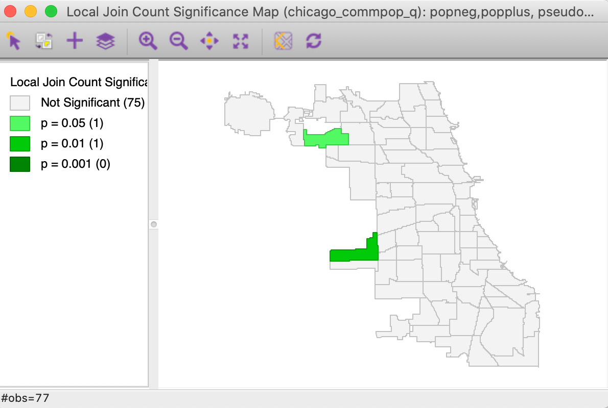
Figure 9: Bivariate Local Join Count significance map

Interpretation

As mentioned earlier, in the current context, the result can be interpreted as evidence of negative spatial autocorrelation, i.e., evidence of spatial outliers. We can illustrate this in our unique values map in Figure 1.

As before, we invoke the option (right click) Connectivity > Show Selection and Neighbors, which outlines the neighbors of a selected observation. With the selection of the most significant location in Figure 9 (the Garfield Ridge community area), its neighbors are highlighted, as shown in Figure 10.

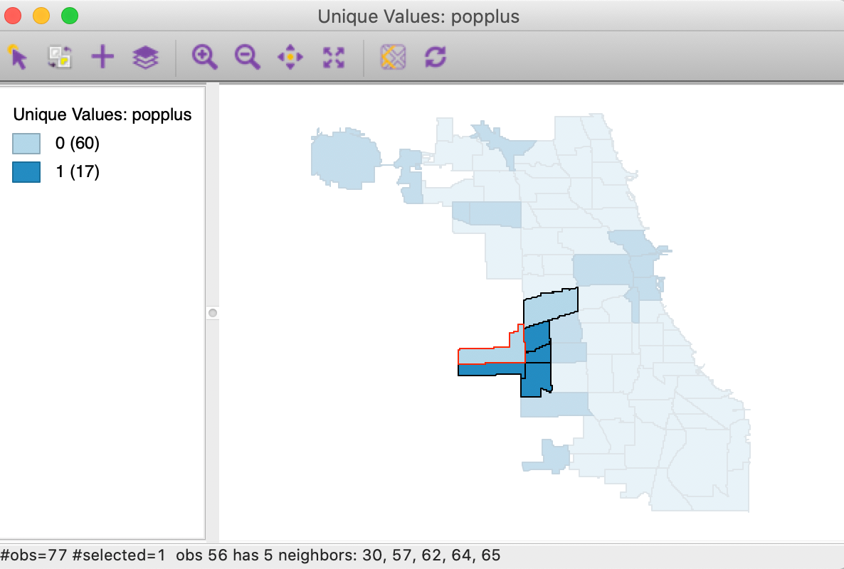
Figure 10: Spatial outlier

In our example, the selected significant area (with negative population change) has a red outline, and is surrounded by one other neighbor with negative population change (light blue), but four neighbors with positive population change (dark blue). Having four of the five neighbors with the opposite sign is sufficient to identify this location as a spatial outlier. However, this should be interpreted with some caution, since the Garfield Ridge community area is at the edge of the data set, and we do not have information (in this data set) on population change that occurred to its north and west.

As is the case for the other local spatial autocorrelation coefficients, the results for each location can be saved to the data table by means of the Save Results option. The same three items are included as for the Univariate Local Join Count statistic: the join count statistic (i.e., the number of neighbors with value \(z_j = 1\)), the total number of neighbors, and the pseudo p-value.

Co-Location Join Count Statistic

Principle

With co-location, the observation at location \(i\) has to have \(x_i = z_i = 1\).

A bivariate co-location cluster requires that an observation for which \(x_i = z_i = 1\) coincides with neighbors for which \(x_j = z_j = 1\) as well. For the bivariate case, the corresponding Local Join Count statistic takes the form (Anselin and Li 2019): \[CLC_i = x_iz_i \sum_j w_{ij}x_jz_j,\] with \(w_{ij}\) as unstandardized (binary) spatial weights. As before, there are \(P\) observations with \(x_i = 1\) and \(Q\) observations with \(z_i = 1\) out of a total of \(n\).

A conditional permutation approach can be constructed for those locations with \(x_i = z_i = 1\). We draw \(k_i\) pairs of observations \((x_j, z_j)\) from the set of \(n−1\) (this contains \(P−1\) observations with \(x_j = 1\) and \(Q−1\) observations with \(z_j = 1\)). In a one-sided test, we again count the number of times the statistic equals or exceeds the observed join count value at \(i\).

The extension to more than two variables is mathematically straightforward. We consider \(k\) variables at each location \(i\), i.e., \(x_{hi}\), for \(h = 1, \dots, k\), with \(\Pi_{h=1}^k x_{hi} = 1\), which enforces the co-location requirement.

The corresponding statistic is then: \[CLC_i = \Pi_{h=1}^k x_{hi} \sum_j w_{ij} \Pi_{h=1}^k x_{hj}.\]

The implementation of a conditional permutation strategy follows as a direct generalization of the bivariate co-location cluster. However, for a large number of variables, such co-locations become less and less likely, and a different conceptual framework may be more appropriate.

Implementation

Preliminaries

To illustrate the co-location case, we will use the Chicago Health data set and the associated CommArea_ACS14_f.shp file. It is again for the 77 Chicago community areas, but contains considerably more socio-economic and health indicators. We will also need a spatial weighs file, such as queen contiguity in CommArea_ACS14_f_q.gal.⁶

We select two particular variables, the number of age-adjusted diabetes-related deaths per 100,000 persons, DiabetM, and the proportion of people with income below 50% of the poverty line, Pov50P.

In Figure 11, we show a quartile map for each variable, suggesting quite similar patterns. Parenthetically, the correlation between the two variables is 0.632.

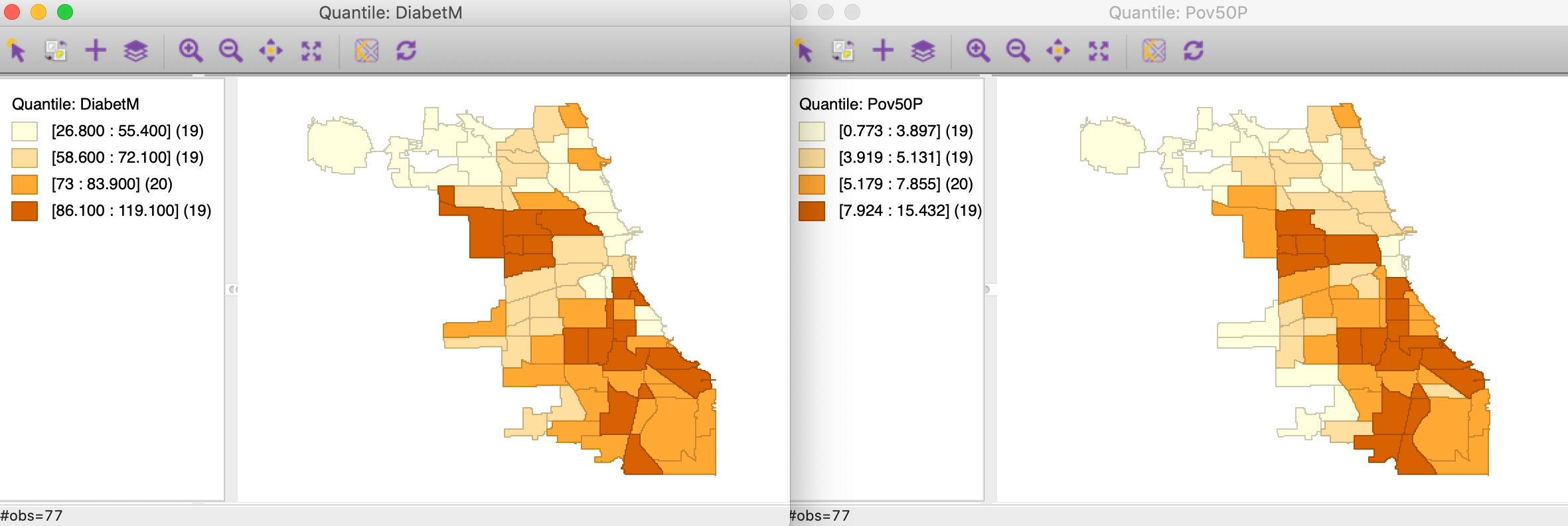
Figure 11: Quartile map - diabetes and poverty

We now convert each continuous variable to an indicator for the upper quartile, with associated variables s_diag and s_pov. These are the binary variables we will consider in our illustration of the co-location local join count test. The associated unique values maps are shown in Figure 12.

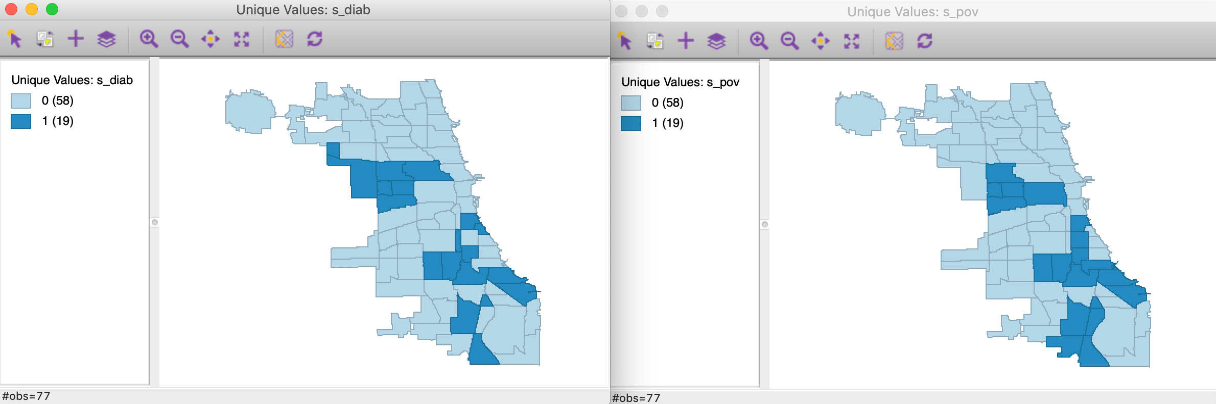
Figure 12: Unique values map - diabetes and poverty upper quartiles

Finally, we assess the overlap between the two spatial patterns in Figure 12 by means of a co-location map, shown in Figure 13. Of the 19 observations in the upper quartile, no less than 14 are shared between the two variables, as shown in Figure 13. Our research question is to assess the extent to which these locations are surrounded by similarly co-located locations, or, in other words, to find spatial clusters of co-location.

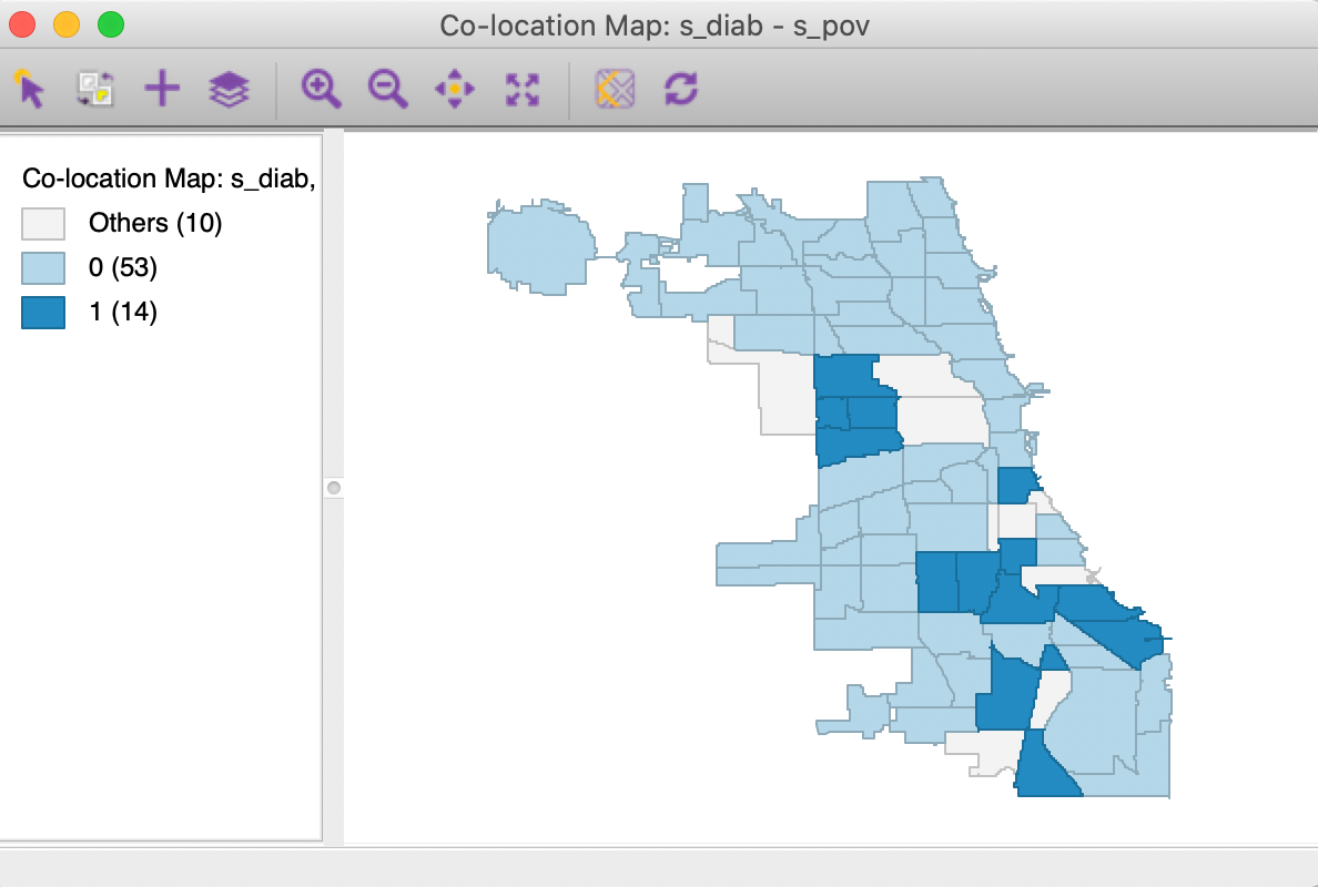
Figure 13: Colocation map - diabetes and poverty upper quartiles

Significance

We invoke the Co-location Local Join Count statistic as the last item in the third group in the Cluster Maps drop down list from the toolbar, shown in Figure 2, or, from the menu, as Space > Co-location Join Count.

Next follows the usual dialog to select the variables and specify the spatial weights, as in Figure 14. We select the just created binary variables, s_diab and s_pov.

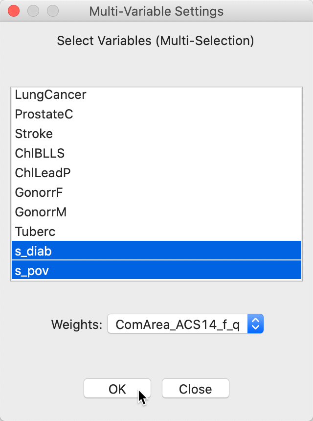
Figure 14: Colocation Local Join Count - Variable selection

This brings up the significance map shown in Figure 15, using the default 999 permutations and p = 0.05. Only three locations out of the 14 co-located observations are (weakly) significant. This suggests that finding actual clusters of co-located observations is much harder in this example than the univariate clusters we encountered so far. In part, this is due to the small number of candidate locations in this example. In larger data sets, this situation can be quite different, as illustrated by the empirical examples in Anselin and Li (2019).

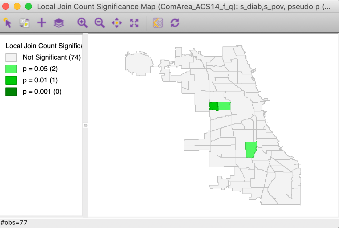
Figure 15: Colocation Local Join Count - significance map

Interpretation

We gain further insight into the actual makeup of the clusters by turning on the Connectivity > Show Selection and Neighbors option in the unique values map and selecting the three significant observations. The result is shown in Figure 16. The selected observations have a red outline and are shown together with their neighbors. Of the two observations that make up the cluster in the western part of the map, one location has three out of its four neighbors as co-locations, whereas the other one has three out of five neighbors. The not co-located observations, in grey color, belong to the upper quartile for one of the variables, but not for both.

The situation is slightly different for the cluster in the south, where three neighbors out of six are also co-located. Two of the other ones do not belong to a top quartile for either variable, whereas one is in the upper quartile for diabetes.

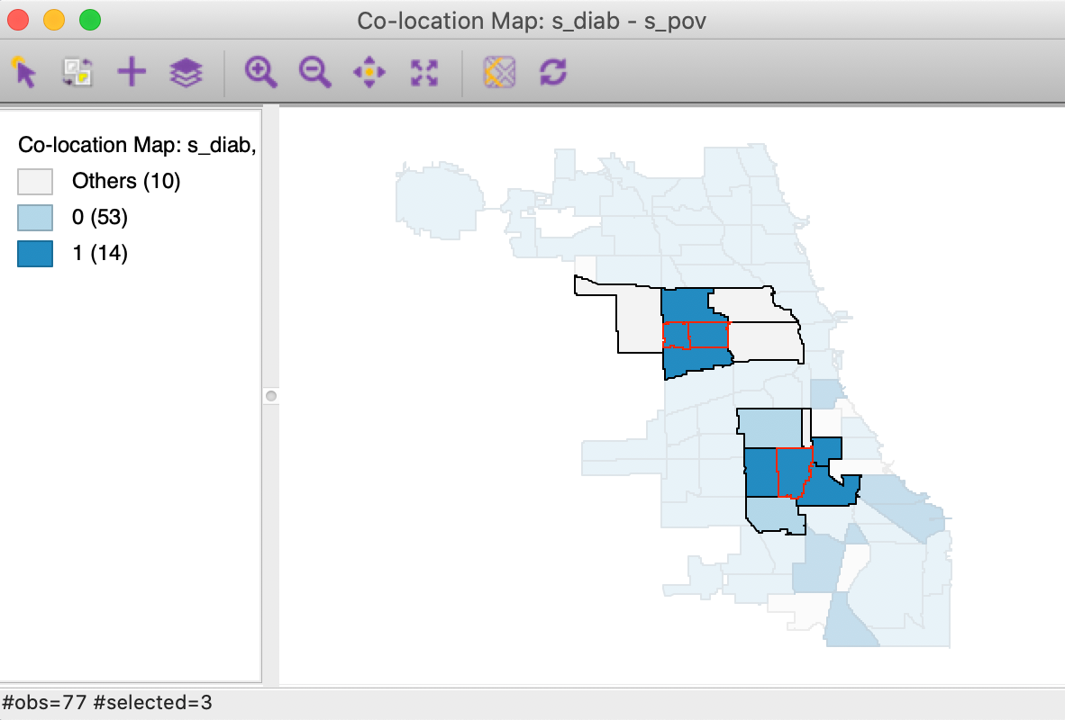
Figure 16: Colocation Local Join Count - clusters

As before, we can Save the results to the table.

Quantile LISA

Principle

The Local Join Count statistics are designed to deal with binary variables. However, as we illustrated with our previous example, they can also be applied to assess the spatial autocorrelation between quantiles of a continuous variable. In Anselin (2019), this is referred to as Quantile LISA or quantile local spatial autocorrelation. In a bivariate or multivariate setting, the quantile LISA often serves as a viable alternative to a Bivariate Local Moran or a Multivariate Local Geary, especially when the focus is on extremes in the distribution.

As we discussed, the continuous (linear) association between two variables that is measured by the Bivariate Local Moran suffers from the problem of in-situ correlation. The quantile local spatial autocorrelation sidesteps this problem by converting the continuous variable to a binary variable that takes the value of 1 for a specific quantile.

For example, as in our previous illustration, the spatial assocation between two continuous variables can be simplified by focusing on the local autocorrelation between binary variables for the upper quartile. Since the bivariate (or multivariate) Local Join Count statistic enforces co-location, the problem of in-situ correlation is controlled for. This provides an alternative to other bivariate and multivariate local spatial autocorrelation statistics, albeit with a loss of information (going from the continuous variable to a binary category).

In addition, the quantile LISA approach can also be employed to assess negative spatial autocorrelation, such as between the upper and lower quantile of a variable. This would be a special case of a No-Colocation Bivariate Local Join Count statistic.

Again, the quantile approach focuses on the extremes of the distributions and thus constitutes a loss of information. However, in practice, this loss of information is often compensated for by superior insight and a focus on the most important interesting locations.

Formally, a continuous variable \(y\) with a cumulative density function \(F(y)\) yields a sequence of ranked observations as \(y_1, y_2, \dots, y_n\). A new binary variable \(x\) is created that takes on the value \(x_i = 1\) for all \(y_i\) for which \(y_{ql} \leq y_i \lt y_{qu}\), with \(y_{ql}\) and \(y_{qu}\) as lower and upper bounds for a given quantile.⁷ For all other observations, \(x_i = 0\).

The new \(x\) variable (or set of such variables in a multivariate case) then forms the basis for a Local Join Count statistic, or one of its multivariate extensions.

Implementation

As we illustrated in the previous example, a quantile LISA can be implemented as a two-step process using the current Local Join Count functionality, with the first step consisting of the creation of the binary variable. The Quantile LISA functionality in GeoDa reduces this to a one step process by employing a specialized variable selection interface.

The functionality is invoked from the next to last group in the Cluster Maps toolbar icon drop down list, in Figure 2, or, from the menu, as Space > Univariate Quantile LISA or Space > Multivariate Quantile LISA.

Univariate Quantile LISA

We continue with the Chicago Health data set and illustrate the univariate case with the example of the upper quartile of the poverty rate, Pov50P. A unique value map for this quartile was given in the left-hand panel of Figure 12.

The variable selection dialog for the univariate case is shown in Figure 17. Beyond specifying a variable name (Pov50P), we also need to set the Number of Quantiles. The default is 5, but in our example, we have set it to 4, for quartiles. In addition, we need to specify the relevant quantile, in Select a Quantile for LISA. The default is 1, but here we have set it to 4, for the upper quartile. Finally, we also need to select a name for the binary variable that will be created, in Save Quantile Selection in Field. We leave the default to QT.

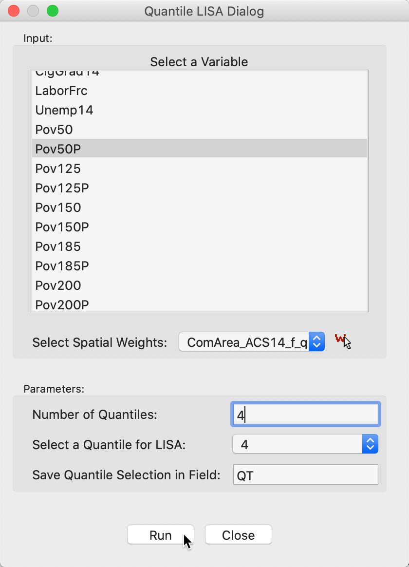
Figure 17: Variable selection - univariate quantile LISA

Using the default settings of 999 permutations and p = 0.05 yields the significance map shown in Figure 18. This identifies 6 locations as significant cores of clusters, but only for p=0.05. The interpretation is the same as that for any other local join count statistic and we do not pursue it further. Also, as before, the results can be saved to the data table.

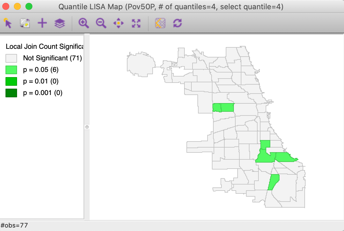
Figure 18: Significance map for Univariate Quantile LISA, poverty rate

Multivariate Quantile LISA

For the multivariate case, the variable selection interface is somewhat more complex, since several aspects need to be specified.

Figure 19 illustrates the various options. First, for each variable, the number of quantiles and the selected one need to be set, as in the univariate case. We have selected the first variable as Pov50P, with the Number of Quantiles set to 4 (the default is 5), and the Quantile for LISA as 4, for the top quartile (1 is the default). In addition, we need to choose a variable name, here QT2. Finally, the combination of options is moved to the right-hand panel by means of the > button.

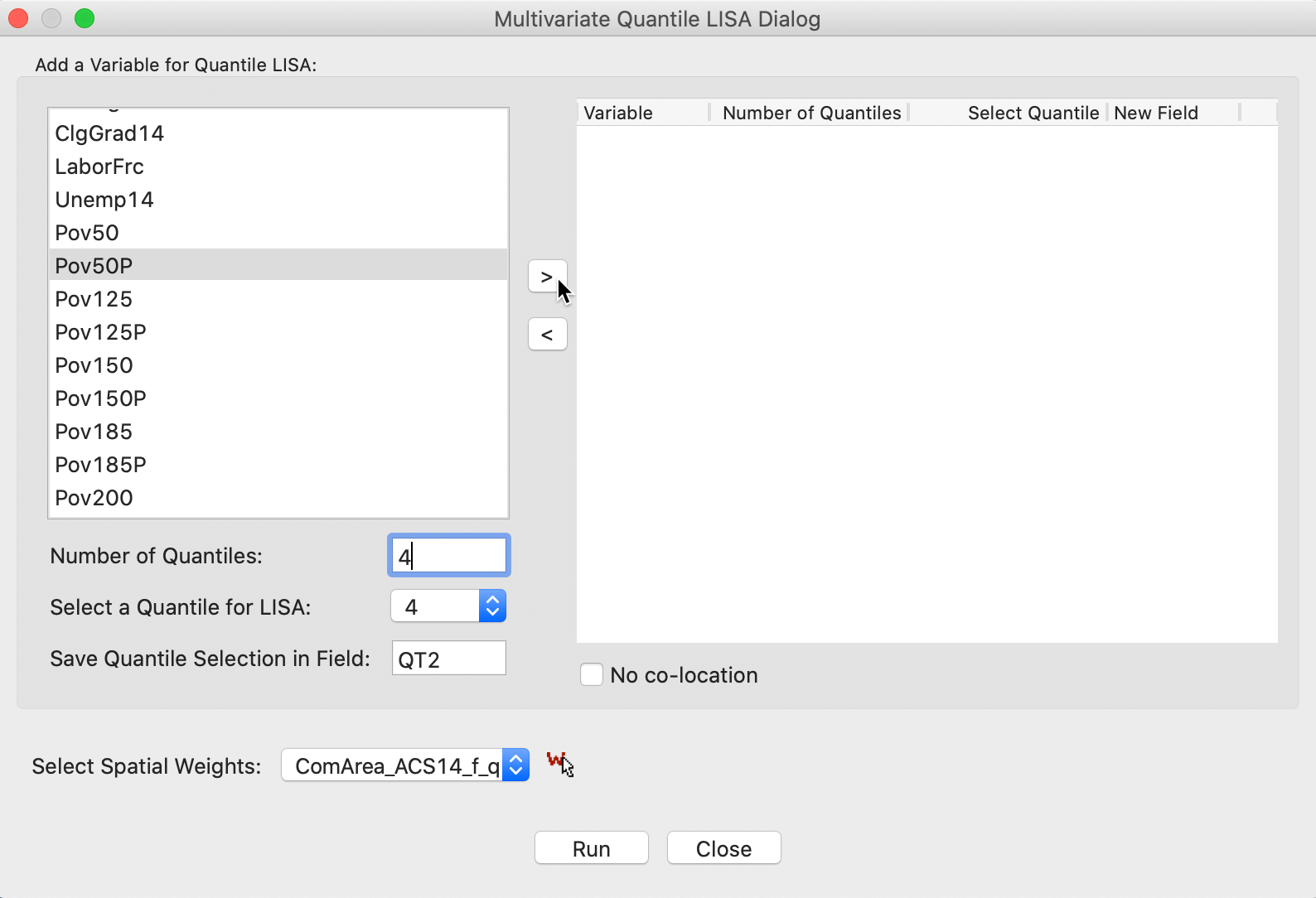
Figure 19: Variable selection - multivariate quantile LISA (1)

With the same settings for the second variable, DiabetM, the right-hand panel is populated as in Figure 20. This interface is completely flexible in the sense that not all variables have to be in the same quantile, but it should be kept in mind that not every combination is meaningful.

The default implementation of the Multivariate Quantile LISA is to compute a Co-Location Multivariate Local Join Count statistic, effectively searching for co-location clusters. Whereas in practice this is the most likely application, the co-location assumption is inappropriate for the analysis of negative spatial autocorrelation, such as between the upper and lower quantile of the same variable. In the interface, this is set by checking the box next to No co-location, as highlighted in Figure 20.

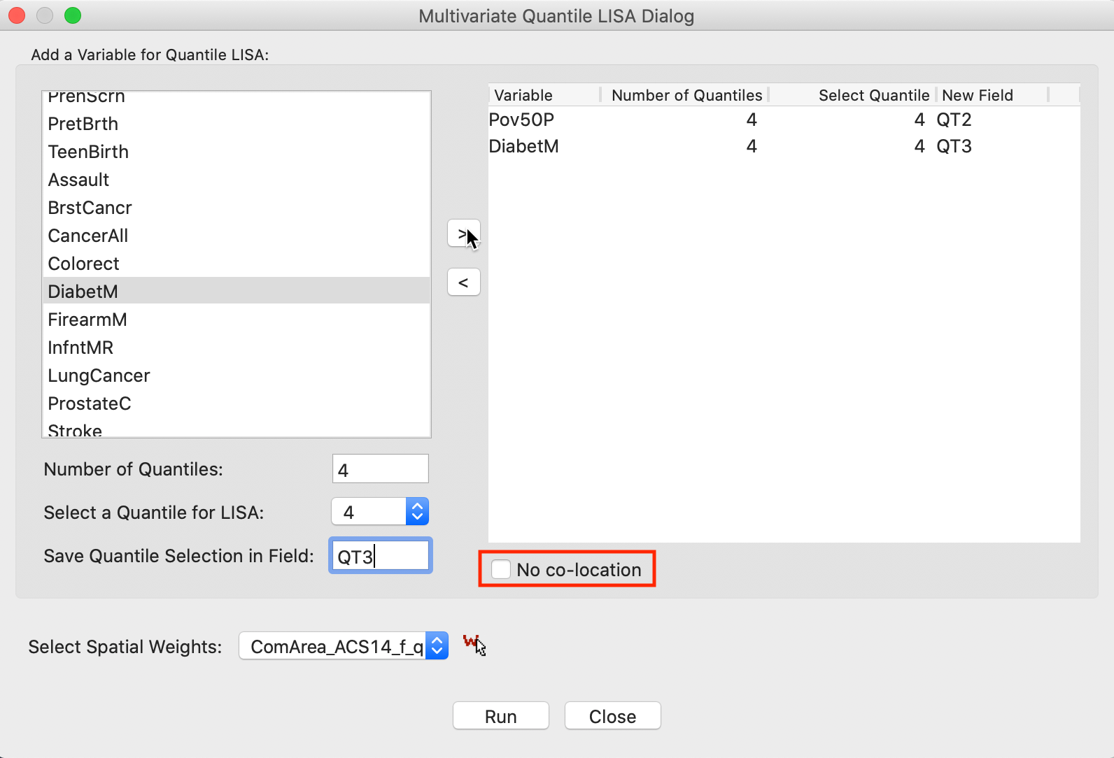
Figure 20: Variable selection - multivariate quantile LISA (2)

With the variable selection as in Figure 20 and the default number of permutations of 999, with p=0.05, the significance map shown in Figure 21 results. This map is identical to the findings shown in Figure 15 for the Co-Location Multivariate Local Join Count computed for the two discrete variables. The only difference is that here the discrete variables are created on the fly, and the window header lists the actual variables with associated quantile information.

In all other respects, the functionality and interpretation are the same as in the multivariate co-location case.

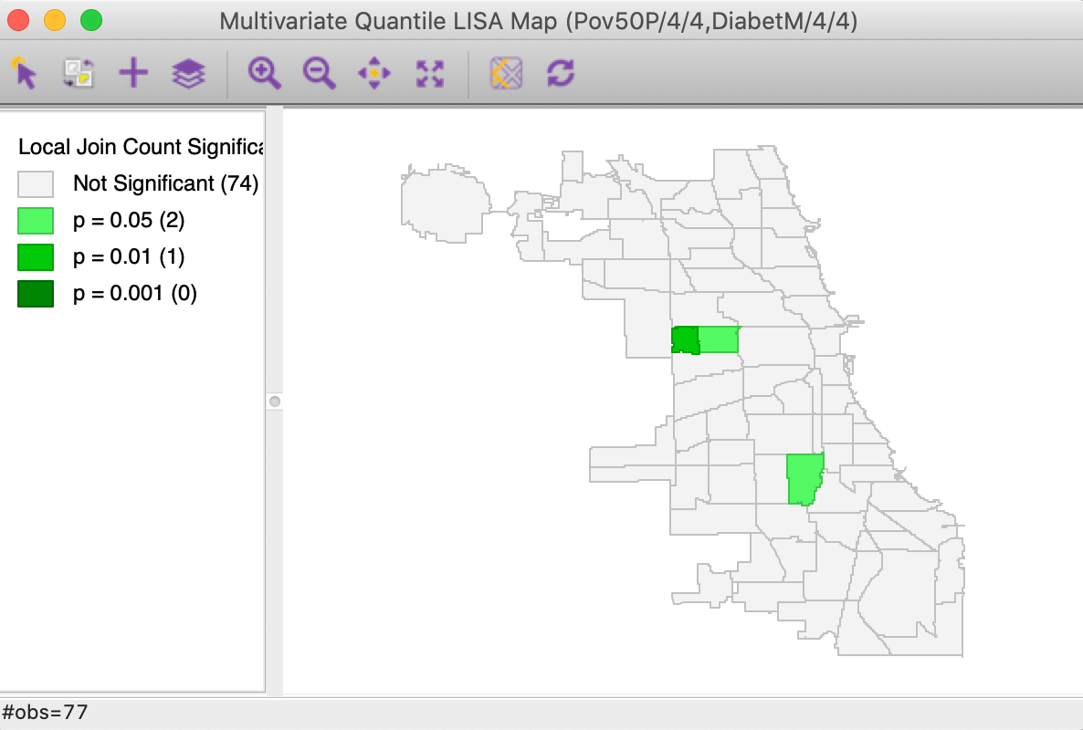
Figure 21: Significance map for Multivariate Quantile LISA, poverty rate and diabetes

References

Anselin, Luc. 1995. “Local Indicators of Spatial Association — LISA.” Geographical Analysis 27: 93–115.

———. 2019. “Quantile Local Spatial Autocorrelation.” Letters in Spatial and Resource Sciences 12 (2): 155–66.

Anselin, Luc, and Xun Li. 2019. “Operational Local Join Count Statistics for Cluster Detection.” Journal of Geographical Systems 21 (2): 189–210.

Cliff, Andrew, and J. Keith Ord. 1973. Spatial Autocorrelation. London: Pion.

Getis, A. 1984. “Interaction Modeling Using Second-Order Analysis.” Environment and Planning A 16 (2): 173–83.

Getis, Arthur, and Janet Franklin. 1987. “Second-Order Neighborhood Analysis of Mapped Point Patterns.” Ecology 68 (3): 473–77.

Getis, Arthur, and J. Keith Ord. 1992. “The Analysis of Spatial Association by Use of Distance Statistics.” Geographical Analysis 24: 189–206.

---

1. University of Chicago, Center for Spatial Data Science – anselin@uchicago.edu↩︎

2. To create the weights matrix, use the variable NID as the ID variable.↩︎

3. In practice, this can easily be detected when the results show locations with 1 like neighbor to be significant, and locations with more like neighbors not to be significant.↩︎

4. Since the permutation test is designed to identify rare occurrences, it will mistakenly flag as significant locations that have fewer neighbors of the predominant type than expected randomly. This is because the proportion of such values in the population is larger than 0.5 so that it is likely to have a large number of neighbors of the type.↩︎

5. For a more meaningful example, see the empirical illustration in Anselin and Li (2019).↩︎

6. The associated ID variable is ComAreaID.↩︎

7. In general, this may be applied to any interval, not just a given quantile.↩︎

GeoDa is maintained by lixun910. This page was generated by GitHub Pages using the Cayman theme by Jason Long.