Cluster Analysis (2)

Hierarchical Clustering Methods

Introduction

In this second chapter on classical clustering methods, we cover hierarchical clustering. In contrast to partioning methods, where the number of clusters (k) needs to be specified a priori, hierarchical clustering methods build up the clusters step by step. The size of the cluster is determined from the results at each step that are visually represented in a tree structure, the so-called dendrogram.

The successive steps can be approached in a top-down fashion or in a bottom-up fashion. The latter is referred to as agglomerative hierarchical clustering, the former as divisive clustering. In this chapter, we will limit our attention to agglomerative methods. A form of divisive clustering is implemented in some of the spatially constrained clustering techniques, which are discussed in a later chapter.

In agglomerative clustering, we start with each observation being assigned to its own cluster (i.e., n clusters of one observation each). Next, the two observations are found that are closest using a specified distance criterion, and they are combined into a cluster. This process repeats itself, by using a representative distance for each grouping once multiple observations are combined. At the end of this process, there is a single cluster that contains all the observations. The result of the successive groupings of the observations is visualized in a dendrogram. A cut point can be applied at any position in the tree to extract the full description of a cluster for all values of \(k\) between \(n\) and 1.

Agglomerative clustering methods differ with respect to the way in which distances between observations and clusters are computed. There are at least seven different ways to implement this. Here, we will focus on the four most commonly used methods: single linkage, complete linkage, average linkage, and Ward’s method (a special form of centroid linkage).

Hierarchical clustering techniques are covered in detail in Chapter 4 of Everitt et al. (2011) and in Chapter 5 of Kaufman and Rousseeuw (2005). A discussion of fast modern algorithms is contained in Müllner (2011) and Müllner (2013).

To illustrate these methods, we will continue to use the Guerry data set on moral statistics in 1830 France, which comes pre-installed with GeoDa.

Objectives

• Understand the principles behind agglomerative clustering

• Distinguish between different linkage functions

• Understand the implications of using different linkage functions

• Interpret a dendrogram for hierarchical clustering

• Carry out sensitivity analysis

GeoDa functions covered

• Clusters > Hierarchical
  • select cut point
  • select linkage function
  • select standardization option
  • select distance metric
  • cluster characteristics
  • mapping the clusters
  • saving the cluster classification

Agglomerative Clustering

Dissimilarity

An agglomerative clustering algorithm starts with each observation serving as its own cluster, i.e., beginning with \(n\) clusters of size 1. Next, the algorithm moves through a sequence of steps, where each time the number of clusters is decreased by one, either by creating a new cluster from two observations, or by assigning an observation to an existing cluster, or by merging two clusters. Such algorithms are sometimes referred to as SAHN, which stands for sequential, agglomerative, hierarchic and non-overlapping (Müllner 2011).

The smallest within-group sum of squares is obtained in the initial stage, where each observation is its own cluster. As soon as two observations are grouped, the within sum of squares increases. Hence, each time a new merger is carried out, the overall objective of minimizing the within sum of squares deteriorates. At the final stage, when all observations are joined into a single cluster, the total within sum of squares equals the total sum of squares. So, whereas partioning cluster methods aim to improve the objective function at each step, agglomerative hierarchical clustering moves in the opposite direction.

The key element in this process is how the dissimilarity (or distance) between two clusters is computed, the so-called linkage. In this chapter, we consider four common types. We discuss single linkage here to illustrate the main concepts and cover the other methods separately below.

For single linkage, the relevant dissimilarity is between the two points in each cluster that are closest together. More precisely, the dissimilarity between clusters \(A\) and \(B\) is: \[d_{AB} = \mbox{min}_{i \in A,j \in B} d_{ij},\] i.e., the nearest neighbor distance between \(A\) and \(B\).

A second important concept is how the distances between other points (or clusters) and a newly merged cluster are computed, the so-called updating formula. With some clever algebra, it can be shown that these calculations can be based on the dissimilarity matrix from the previous step and do not require going back to the original \(n \times n\) dissimilarity matrix.² Note that at each step, the dimension of the relevant dissimilarity matrix decreases by one, which allows for very memory-efficient algorithms.

In the single linkage case, the updating formula takes a simple form. The dissimilarity between a point (or cluster) \(P\) and a cluster \(C\) that was obtained by merging \(A\) and \(B\) is the smallest of the dissimilarities between \(P\) and \(A\) and \(P\) and \(B\): \[d_{PC} = \mbox{min}(d_{PA},d_{PB}),\] using the definition of dissimilarity between two objects (\(d_{AB}\)) given above.

The minimum condition can also be obtained as the result of an algebraic expression: \[d_{PC} = (1/2) (d_{PA} + d_{PB}) - (1/2)| d_{PA} - d_{PB} |,\] in the same notation as before.³

The updating formula only affects the row/column in the dissimilarity matrix that pertains to the newly merged cluster. The other elements of the dissimilarity matrix remain unchanged.

Single linkage clusters tend to result in a few clusters consisting of long drawn out chains of observations as well as several singletons (observations that form their own cluster). This is due to the fact that sometimes disparate clusters are joined when they have two close points, but otherwise are far apart. Single linkage is sometimes used to detect outliers, i.e., observations that remain singletons and thus are far apart from all others.

Illustration: single linkage

To illustrate the logic of agglomerative hierarchical clustering algorithms, we use the example of single linkage applied to the same seven points as we used for k-means. For ease of reference, the points are shown in Figure 1.⁴ As before, the point IDs are ordered with increasing values of X first, then Y, starting with observation 1 in the lower left corner. Full details are given in the Appendix.

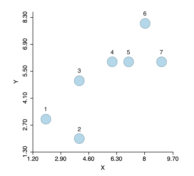
Figure 1: Single link hierarchical clustering toy example

The basis for any agglomerative clustering method is a \(n \times n\) symmetric dissimilarity matrix. Except for Ward’s method, this is the only information needed. In our example, we use a dissimilarity matrix based on the Euclidean distances between the points, as shown in Figure 2

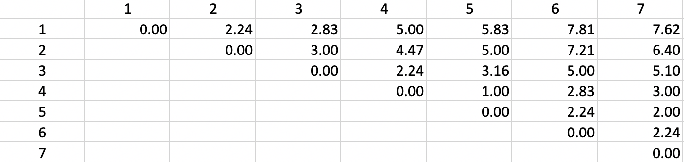
Figure 2: Dissimilarity matrix

The first step is to identify the pair of observations that have the smallest nearest neighbor distance. From the distance matrix and also from Figure 3 this is the pair 4-5 (\(d_{4,5}=1.0\)). This forms the first cluster, highlighted in dark blue in the figure. The five other observations remain in their own cluster. In other words, at this stage, we still have six clusters.

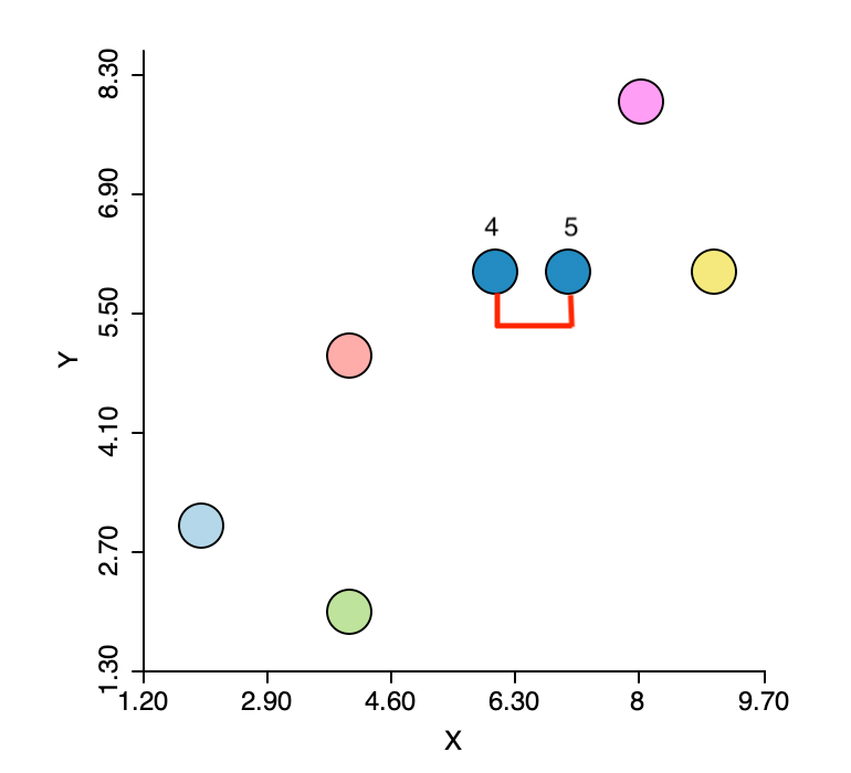
Figure 3: Nearest neighbors

The algorithm then moves sequentially to identify the nearest neighbor at each step, merge the relevant observations/clusters and so decrease the number of clusters by one. The steps are illustrated in the panels of Figure 4, going from left to right and starting at the top. In the second step, another observation (7) is added to the 4,5 cluster. Next, a new cluster emerges consisting of 1 and 2 (the two green points in the lower left). Finally, first 3 and then 6 are added to the large blue cluster. Details are given in the Appendix.

Figure 4: Single linkage iterations

Dendrogram

The agglomerative nesting is visually represented in a tree structure, the so-called dendrogram. For each step, the graph shows which observations/clusters are combined. In addition, the different horizontal extents (i.e., how far each cluster combination is from the right side of the graph) give a sense of the degree of change in the objective function achieved by each merger.

The implementation of the dendrogram in GeoDa is currently somewhat limited, but it accomplishes the main goal. In Figure 5, the result is shown for single linkage in our toy example. The graph shows how the cluster starts by combining two observations (4 and 5), to which then a third (7) is added. These first two steps are highlighted in the dendrogram and the corresponding observations are selected in the Table.

Next, following the tree structure reveals how two more observations (1 and 2) are combined into a separate cluster, and two observations (3 and 6) are added to the original cluster of 4,5 and 7. The fact that the last three operations all line up (same distance from the right side) follows from a three-way tie in the inter-group distances (see the Appendix). As a result, the change in the objective function (more precisely, a deterioration) that follows from adding the points to a cluster is the same in each case.

The dashed vertical line represents a cut line. It corresponds with a particular value of k for which the make up of the clusters and their characteristics can be further investigated (see the section on Cluster results for details on the implementation in GeoDa).

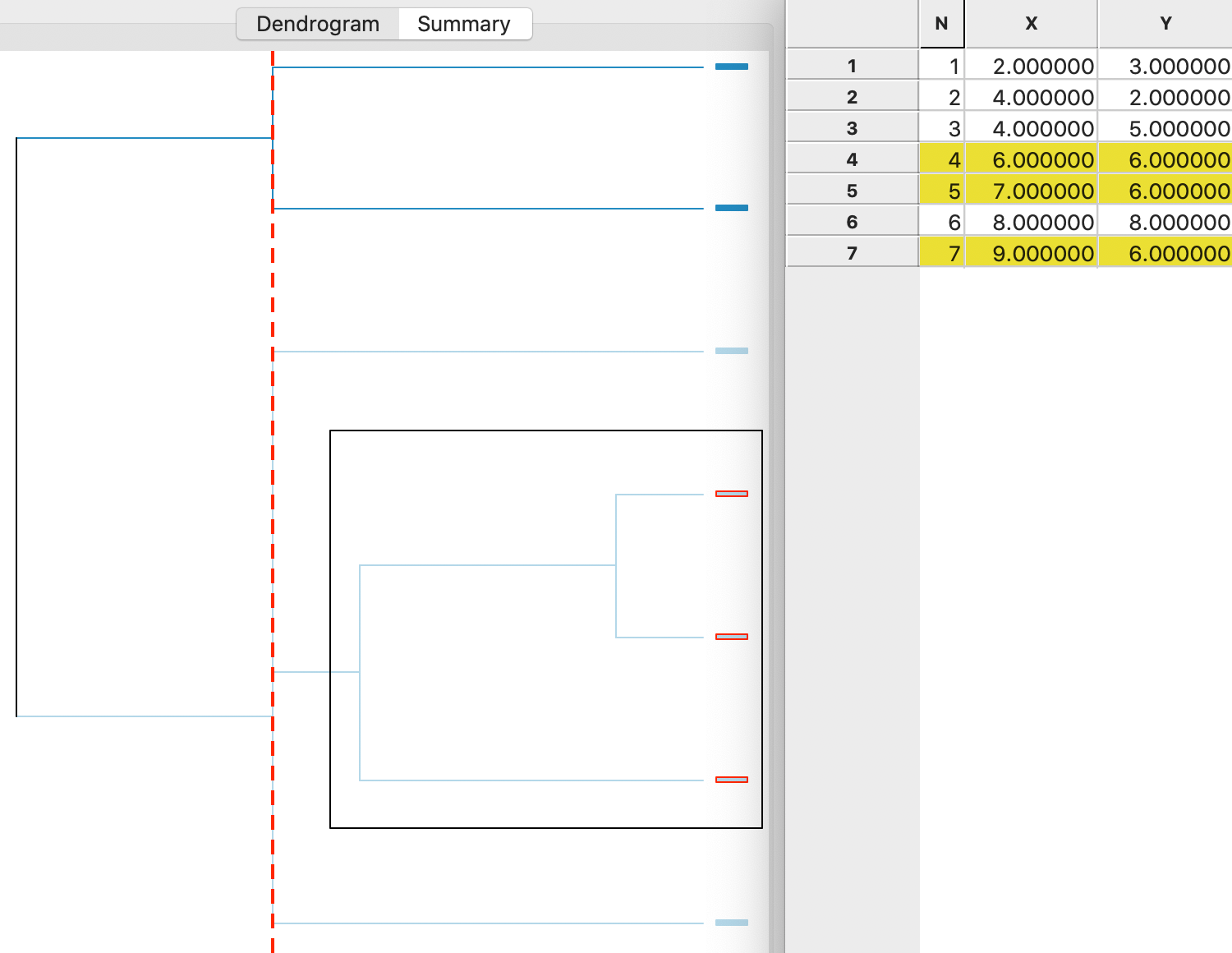
Figure 5: Single linkage dendrogram

Complete linkage

Complete linkage is the opposite of single linkage in that the dissimilarity between two clusters is defined as the furthest neighbors, i.e., the pair of points, one from each cluster, that are separated by the greatest dissimilarity. For the dissimilarity between clusters \(A\) and \(B\), this boils down to: \[d_{AB} = \mbox{max}_{i \in A,j \in B} d_{ij}.\]

With this measure of dissimilarity in hand, we still continue to combine the two observations/clusters that are closest at each step. The only difference with single linkage is how the respective distances are calculated.

The updating formula similarly is the opposite of the one for single linkage. The dissimilarity between a point (or cluster) \(P\) and a cluster \(C\) that was obtained by merging \(A\) and \(B\) is the largest of the dissimilarities between \(P\) and \(A\) and \(P\) and \(B\): \[d_{PC} = \mbox{max}(d_{PA},d_{PB}).\]

The algebraic counterpart of the updating formula is: \[d_{PC} = (1/2) (d_{PA} + d_{PB}) + (1/2)| d_{PA} - d_{PB} |,\] using the same logic as in the single linkage case.

A detailed worked example for complete linkage using our toy data is given in the Appendix. A summary is provided in the dendrogram in Figure 6. This shows the first cluster as observations 4,5. The next steps are to combine 1 and 2 (at the bottom) and 6 and 7 (at the top). In the last two steps, 3 is added to 1,2 and 4,5 and 6,7 are merged (see the Appendix for details).

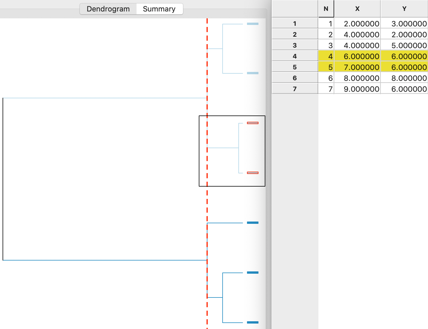
Figure 6: Complete linkage dendrogram

In contrast to single linkage, complete linkage tends to result in a large number of well-balanced compact clusters. Instead of merging fairly disparate clusters that have (only) two close points, it can have the opposite effect of keeping similar observations in separate clusters.

Average linkage

In average linkage, the dissimilarity between two clusters is the average of all pairwise dissimilarities between observations \(i\) in cluster \(A\) and \(j\) in cluster \(B\). There are \(n_A.n_B\) such pairs (only counting each pair once), with \(n\) as the number of observations in each cluster. Consequently, the dissimilarity between \(A\) and \(B\) is: \[d_{AB} = \frac{\sum_{i \in A} \sum_{j \in B} d_{ij}}{n_A.n_B}.\] Note that when merging two single observations, \(d_{AB}\) is simply the dissimilarity between the two, since \(n_A = n_B = 1\) and the denominator in the expression is 1.

The updating formula to compute the dissimilarity between a point (or cluster) \(P\) and the new cluster \(C\) formed by merging \(A\) and \(B\) is the weighted average of the dissimilarities \(d_{PA}\) and \(d_{PB}\): \[d_{PC} = \frac{n_A}{n_A + n_B} d_{PA} + \frac{n_B}{n_A + n_B} d_{PB}.\] As before, the other distances are not affected.⁵

A detailed worked example for complete linkage using our toy data is given in the Appendix. A summary is provided in the dendrogram in Figure 7. This shows the first cluster again as observations 4,5. As in the case of complete linkage, the next steps are to combine 1 and 2 (at the bottom) and 6 and 7 (at the top). In the last two steps, first 4,5 and 6,7 are merged and then 3 is added to 1,2, in the reverse order of what happened for complete linkage (see the Appendix for details).

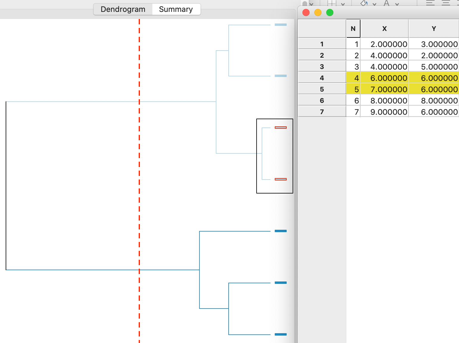
Figure 7: Average linkage dendrogram

Average linkage can be viewed as a compromise between the nearest neighbor logic of single linkage and the furthest neighbor logic of complete linkage. In our example, the end results are almost the same as for complete linkage. However, in general, average linkage tends to produce a few large clusters and many singletons, similar to the results for single linkage (see also the results for the Guerry data shown below).

Ward’s method

The three linkage methods discussed so far only make use of a dissimilarity matrix. How this matrix is obtained does not matter. As a result, dissimilarity may be defined using Euclidean or Manhattan distance, dissimilarity among categories, or even directly from interview or survey data.

In contrast, the method developed by Ward (1963) is based on a sum of squared errors rationale that only works for Euclidean distance between observations. In addition, the sum of squared errors requires the consideration of the so-called centroid of each cluster, i.e., the mean vector of the observations belonging to the cluster. Therefore, the input into Ward’s method is a \(n \times p\) matrix \(X\) of actual observations on \(p\) variables (as before, this is typically standardized in some fashion).

Ward’s method is based on the objective of minimizing the deterioration in the overall within sum of squares. The latter is the sum of squared deviations between the observations in a cluster and the centroid (mean), as we have seen before in k-means clustering: \[WSS = \sum_{i \in C} (x_i - \bar{x}_C)^2,\] with \(\bar{x}_C\) as the centroid of cluster \(C\).

Since any merger of two existing clusters (including individual observations) results in a worsening of the overall WSS, Ward’s method is designed to minimize this deterioration. More specifically, it is designed to minimize the difference between the new (larger) WSS in the merged cluster and the sum of the WSS of the components that were merged. This turns out to boil down to minimizing the distance between cluster centers.⁶ This is reminiscent of the equivalence between Euclidean distances and sum of squared errors we saw in the discussion of k-means. As in k-means, we work with the square of the Euclidean distance: \[d_{AB}^2 = \frac{2n_A n_B}{n_A + n_B} ||\bar{x}_A - \bar{x}_B ||^2,\] where \(||\bar{x}_A - \bar{x}_B ||\) is the Euclidean distance between the two cluster centers (squared in the distance squared expression).⁷

The hierarchical nesting steps proceed in the same way as for the other methods, by merging the two observations/clusters that are the closest, but now based on a more complex distance metric.

The update equation to compute the (squared) distance from an observation (or cluster) \(P\) to a new cluster \(C\) obtained from the merger of \(A\) and \(B\) is more complex than for the other linkage options: \[d^2_{PC} = \frac{n_A + n_P}{n_C + n_P} d^2_{PA} + \frac{n_B + n_P}{n_C + n_P} d^2_{PB} - \frac{n_P}{n_C + n_P} d^2_{AB},\] in the same notation as before. However, it can still readily be obtained from the information contained in the dissimilarity matrix from the previous step, and it does not involve the actual computation of centroids.

To see why this is the case, consider the usual first step when two single observations are merged. The distance squared between them is simply the Euclidean distance squared between their values, not involving any centroids. The updated squared distances between other points and the two merged points only involve the point-to-point squared distances \(d^2_{PA}\), \(d^2_{PB}\) and \(d^2_{AB}\), no centroids. From then on, any update uses the results from the previous distance matrix in the update equation.

A detailed worked example for Ward’s method using our toy data is given in the Appendix. A summary is provided in the dendrogram in Figure 8. This shows the first cluster again as observations 4,5. As in the case of complete linkage, the next steps are to combine 1 and 2 (at the bottom of the graph) and 6 and 7 (at the top of the graph). In the last two steps, as in complete linkage, 3 is first added to 1,2 and then 4,5 and 6,7 are merged (see the Appendix for details).

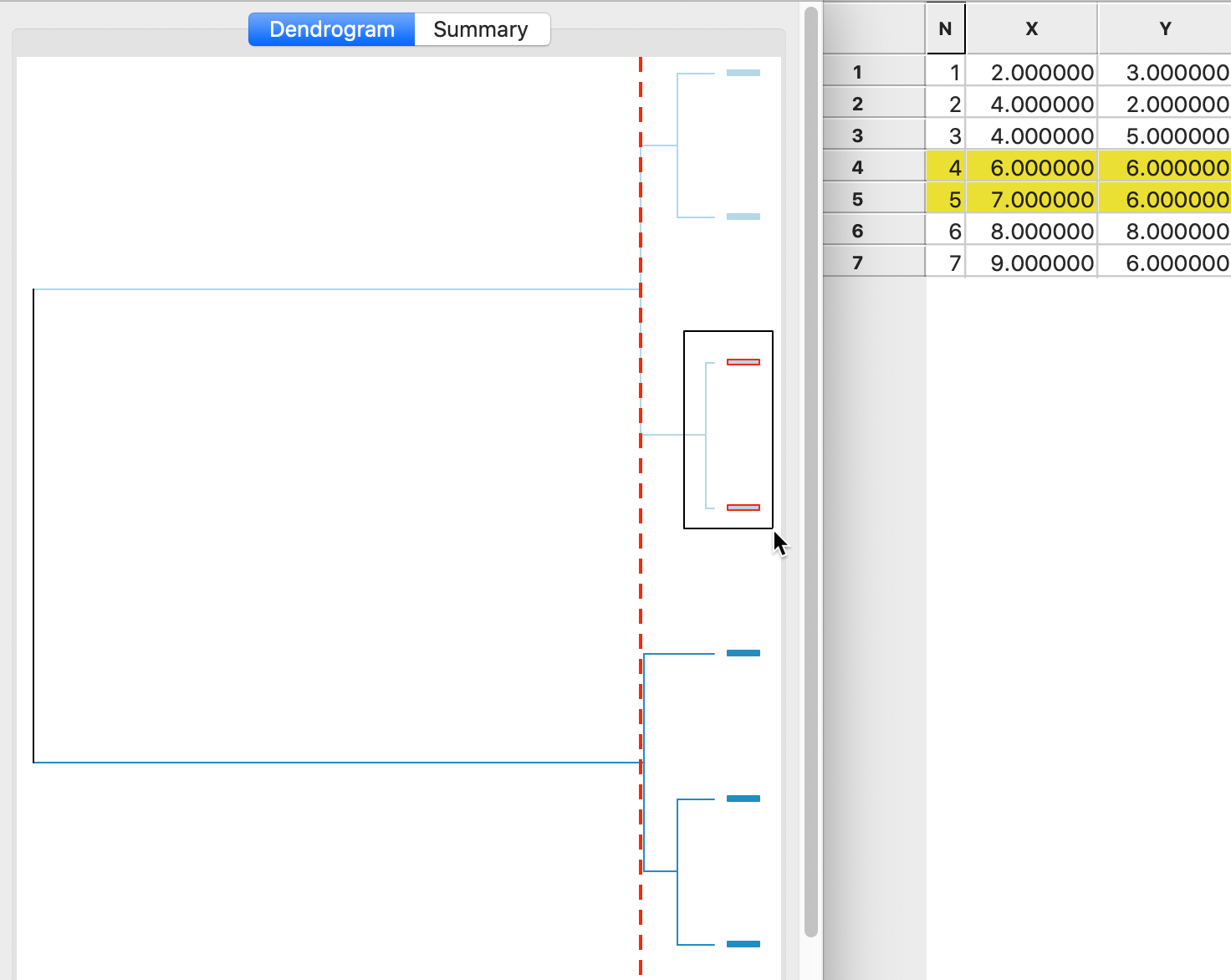
Figure 8: Ward linkage dendrogram

Ward’s method tends to result in nicely balanced clusters. It is therefore set as the default method in GeoDa.

Implementation

Hierarchical clustering is invoked in GeoDa from the same toolbar icon as the other clustering methods. It is the last item in the classic methods subset, as shown in Figure 9. It can also be selected from the menu as Clusters > Hierarchical.

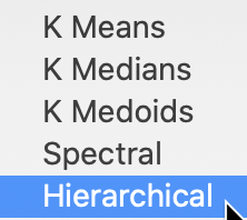
Figure 9: Hierarchical clustering option

Variable Settings Panel

As before, the variables to be clustered are selected in the Variables Settings panel. We continue with the same six variables as for k-means, shown in Figure 10.

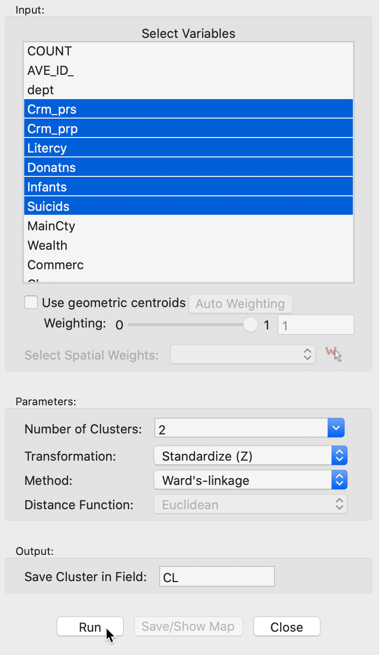
Figure 10: Hierarchical clustering variable selection

The panel also allows one to set the usual options, such as the Transformation (default value is a standardized z-value), and the linkage Method (default is Ward’s linkage). The Distance Function option is not available for the default Ward’s linkage shown here (only Euclidean distance is allowed for this linkage), However, Manhattan distance is an option for the other linkage methods. In the same way as for k-means, the cluster classification is saved in the data table under the variable name specified in Save Cluster in Field.

Cluster results

The actual computation of the clusters proceeds in two steps. In the first step, a click on Run yields a dendrogram in the panel on the right. A cut point can be selected interactively, of by setting a value the number of clusters in the panel. After this, Save/Show Map creates the cluster map, computes the summary characteristics, and saves the cluster classification in the data table.

Dendrogram

With all options set to the default, the resulting dendrogram is as in Figure 11. The dashed red line corresponds to a cut point that yields five clusters, to keep the results comparable with what we obtained for k-means. The dendrogram shows how individual observations are combined into groups of two, and subsequently into larger and larger groups, by merging pairs of clusters. The colors on the right hand side match the colors of the observations in the cluster map (see next). A selection rectangle allows one to select specific groups of observations in the dendrogram. Through linking, the matching observations are identified in the cluster map (and in any graph or map currently open).

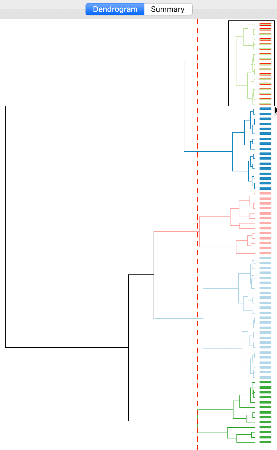
Figure 11: Dendrogram (k=5)

The dashed line (cut point) can be moved interactively. For example, in Figure 12, we grabbed the line at the top (it can equally be grabbed at the bottom), and moved it to the right to yield eight clusters. The corresponding colors are shown on the right hand bar.

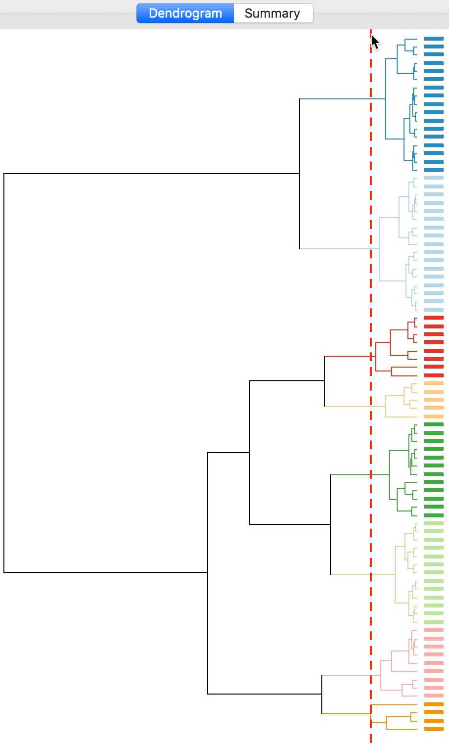
Figure 12: Dendrogram (k=8)

Cluster map

As mentioned before, once the dendrogram cut point is specified, clicking on Save/Show Map will generate the cluster map, shown in Figure 13. Note how the colors for the map categories match the colors in the dendrogram. Also, the number of observations in each class also are the same between the groupings in the dendrogram and the cluster map.

The default Ward’s method yields fairly balanced clusters with two groups with 13 observations, one with 25, and two more with 17. The results show some similarity with the outcome of k-means for k=5, although there are some important differences as well.

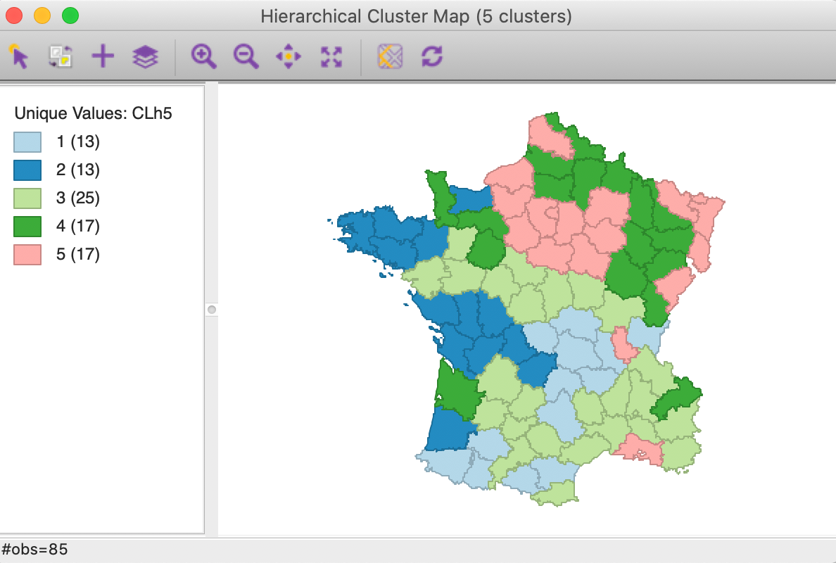
Figure 13: Hierarchical cluster map (Ward, k=5)

Cluster summary

Similarly, once Save/Show Map has been selected, the cluster descriptive statistics become available from the Summary button in the dialog. The same characteristics are reported as for k-means. In comparison to our k-means solution, this set of clusters is slightly inferior in terms of the ratio of between to total sum of squares, achieving 0.482044 (compared to 0.497). Clusters 4 and 5 achieve much better (smaller) within sum of squares than in the k-means solution, but the other values are worse.

Setting the number of clusters at five is by no means necessarily the best solution. In a real application of hierarchical clustering, one would experiment with different cut points and evaluate the solutions relative to the k-means solution.

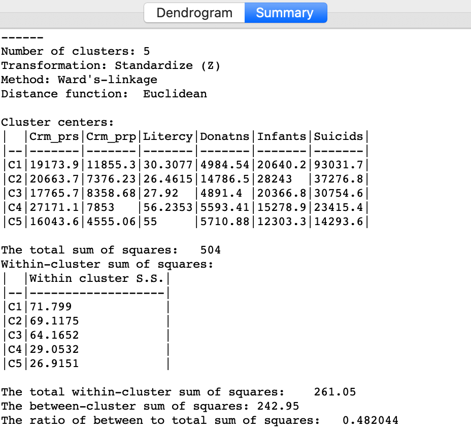
Figure 14: Hierarchical cluster characteristics (Ward, k=5

The two clustering approaches can also be used in conjunction with each other. For example, one could explore the dendrogram to find a good cut-point, and then use this value for k in a k-means or other partitioning method.

Linkage method

The main option of interest in hierarchical clustering is the linkage Method. So far, we have used the default setting for Ward’s-linkage. We now consider each of the other linkage options in turn and illustrate the associated dendrogram, cluster map and cluster characteristics.

Single linkage

The linkage options are chosen from the Method item in the dialog. For example, in Figure 15, we select Single-linkage. The other options are chosen in the same way.

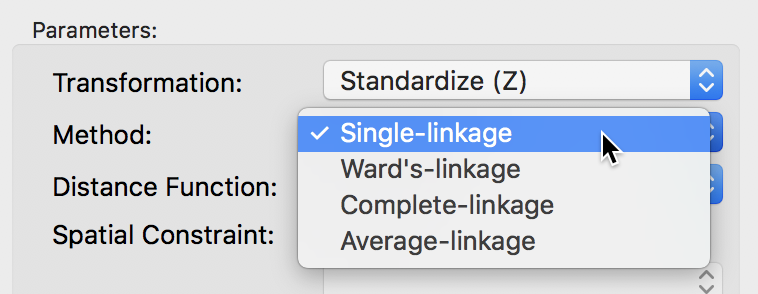
Figure 15: Single linkage

The cluster results for single linkage are typically characterized by one or a few very large clusters and several singletons (one observation per cluster). This characteristic is confirmed in our example, with the dendrogram in Figure 16, and the corresponding cluster map in Figure 17.

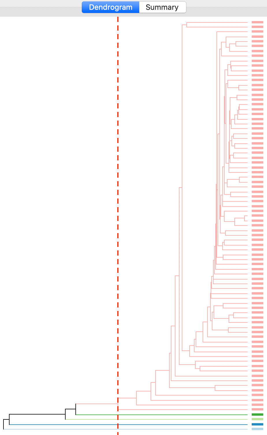
Figure 16: Dendrogram single linkage (k=5)

Four clusters consist of a single observation, with the main cluster collecting the 81 other observations. This situation is not remedied by moving the cut point such that more clusters result, since almost all of the additional clusters are singletons as well.

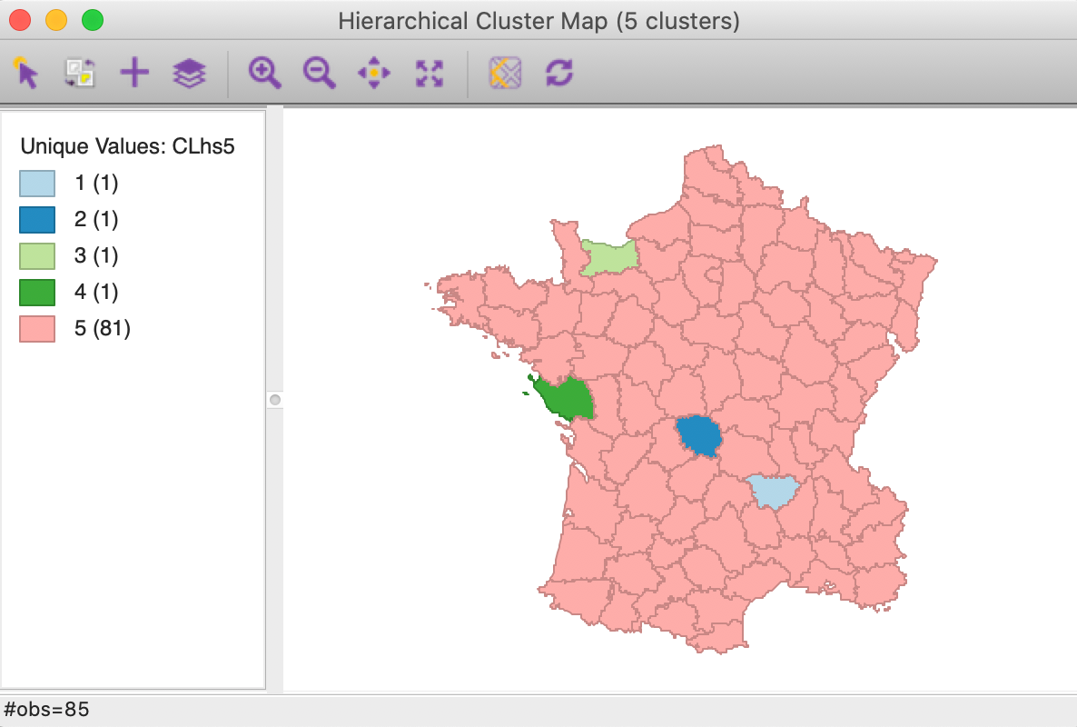
Figure 17: Hierarchical cluster map (single linkage, k=5)

The characteristics of the single linkage hierarchical cluster are similarly dismal. Since four clusters are singletons, their within cluster sum of squares is 0. Hence, the total within-cluster sum of squares equals the sum of squares for cluster 5. The resulting ratio of between to total sum of squares is only 0.214771.

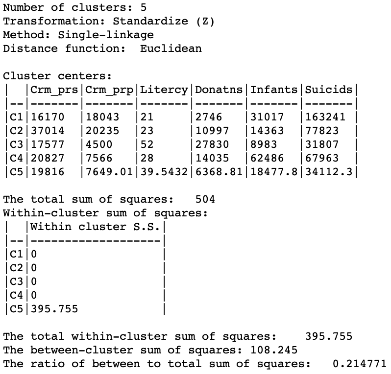
Figure 18: Hierarchical cluster characteristics (single linkage, k=5)

In practice, in most situations, single linkage will not be a good choice, unless the objective is to identify a lot of singletons and characterize these as outliers.

Complete linkage

The complete linkage method yields clusters that are similar in balance to Ward’s method. For example, in Figure 19, the dendrogram is shown for our example, using a cut point with five clusters. The clusters are fairly balanced, unlike what we just saw for single linkage.

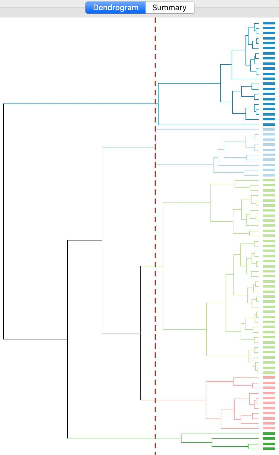
Figure 19: Dendrogram complete linkage (k=5)

The corresponding cluster map is given as Figure 20. The map is similar in structure to that obtained with Ward’s method (Figure 13), but note that the largest category (at 39) is much larger than the largest for Ward (25).

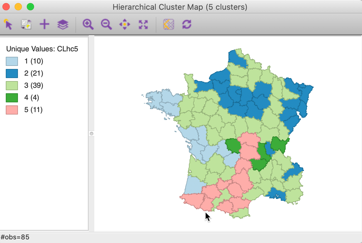
Figure 20: Hierarchical cluster map (complete linkage, k=5)

In terms of the cluster characteristics, shown in Figure 21, we note a slight deterioration relative to Ward’s results, with the ratio of between to total sum of squares at 0.423101 (but much better than single linkage).

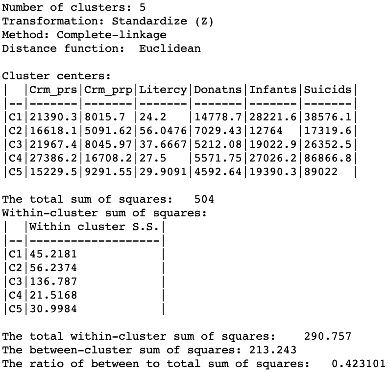
Figure 21: Hierarchical cluster characteristics (complete linkage, k=5)

Average linkage

Finally, the average linkage criterion suffers from some of the same problems as single linkage, although it yields slightly better results. The dendrogram in Figures 22 indicates a similar unbalanced structure, although only with two singletons. The other small clusters consist of two and five observations.

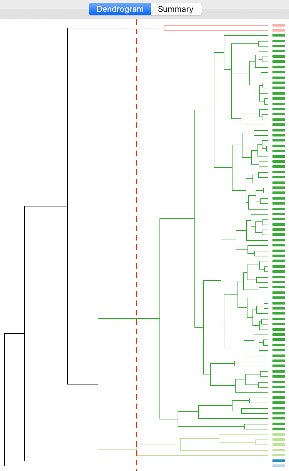
Figure 22: Dendrogram average linkage (k=5)

The cluster map is given as Figure 23. It reinforces that the average linkage criterion is not conducive to discovering compact clusters, but rather lumps most of the observations into one large cluster, with a few outliers.

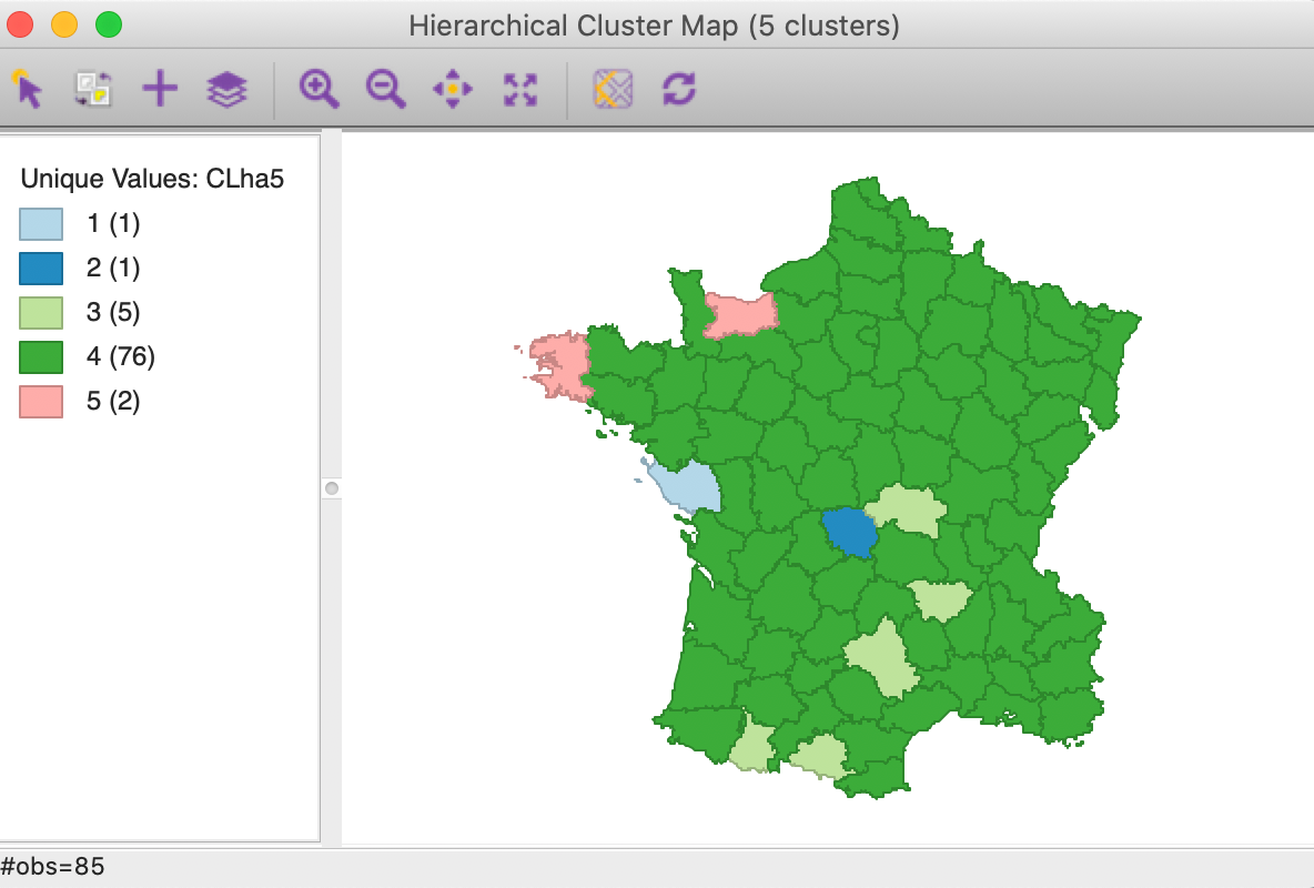
Figure 23: Hierarchical cluster map (average linkage, k=5)

As given in Figure 24, the summary characteristics are slighly better than in the single linkage case, with only two singletons. However, the overall ratio of between to total sum of squares is still much worse than for the other two methods, at 0.296838.

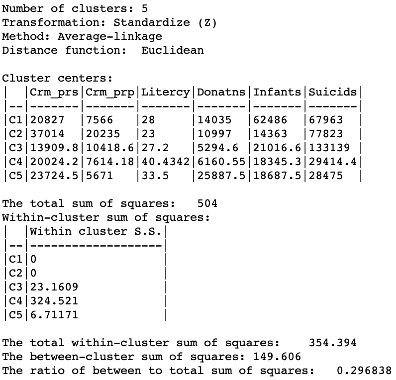
Figure 24: Hierarchical cluster characteristics (average linkage, k=5)

Options and sensitivity analysis

The options are essentially the same for all clustering methods. We can change the Transformation and select a different Distance Function. We briefly consider the latter. However, this option is not appropriate for Ward’s method, which only applies to Euclidean distances.

The option to include a minimum bound is not appropriate for agglomerative clustering, since it would preclude any individual observations to be merged. None would satisfy the minimum bound, unless it was set at a level that was meaningless as a constraint.

Conditional plots, aggregation and dissolution of the cluster results operate in exactly the same way as for k-means clustering and is not covered here.

Distance metric

The default metric behind the definition of dissimilarity is the Euclidean distance between observations. In some contexts, it may be preferable to use absolute or Manhattan block distance, which penalizes larger distances less. This option can be selected through the Distance Function item in the dialog, as in Figure 25, where we choose it for a Complete Linkage clustering (the next best method after Ward’s).

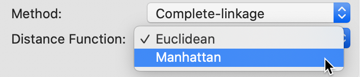
Figure 25: Manhattan distance metric

The cluster map for a cut point of k=5 is shown in Figure 26. Compared to the map for Euclidean distance in Figure 20, some of the configurations are quite different. Two of the clusters are much smaller, but the largest ones are well balanced.

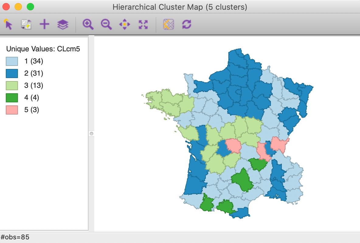
Figure 26: Manhattan distance cluster map

The summary characteristics given in Figure 27. Relative to the Euclidean distance results, some the within sum or squares are much larger, although the largest is not as large as in the Euclidean case, and the smallest is smaller. Also, the ratio of between to total sum of squares is somewhat worse for Manhattan distance, at 0.412 (compared to 0.423). However, this is not a totally fair comparison, since the criterion for grouping is not based on a sum of squared deviations.

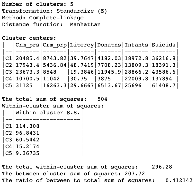
Figure 27: Manhattan distance cluster characteristics

As in the discussion of k-means, it cannot be emphasized enough that the interpretation and choice of the proper cluster is both an art and a science. Considerable experimentation is needed to get good insight into the characteristics of the data and what groupings make the most sense.

Appendix

Single linkage worked example

We now illustrate each step in detail as the single linkage hierarchical cluster algorithm processes our toy example. For ease of reference, the point coordinates (the same as for the k-means example) are listed again in Figure 28. The associated dissimilarity matrix, based on the Euclidean distance between the points (not the squared distance) is given in Figure 2.

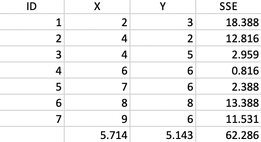
Figure 28: Worked example - basic data

The first step consists of identifying the two observations that are the closest. From the dissimilarity matrix, we find the shortest dissimilarity to be a value of 1.0 between 4 and 5, as highlighted in Figure 29. As a result, 4 and 5 form the first cluster.

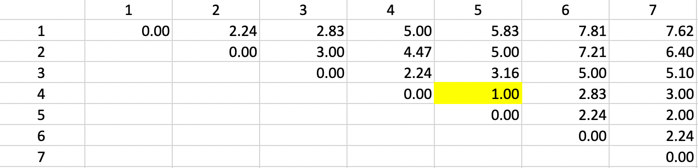
Figure 29: Single Linkage - Step 1

We update the dissimilarity matrix using the smallest dissimilarity between each observation and either 4 or 5 as the entry for the combined unit 4,5. More precisely, the dissimilarity used between the cluster and the other observations varies depending on whether 4 or 5 is closest to the other observations. For example, in Figure 30, we list the dissimilarity between 4,5 and 1 as 5.0, wich is the smallest of 1-4 (5.0) and 1-5 (5.83). The dissimilarities between the pairs of observations that do not involve 4,5 are not affected.

We update the other entries for 4,5 in the same way and again locate the smallest dissimilarity in the matrix. This time, it is a dissimilarity of 2.0 between 4,5 and 7 (more precisely, between 5 and 7). Consequently, observation 7 is added to the 4,5 cluster.

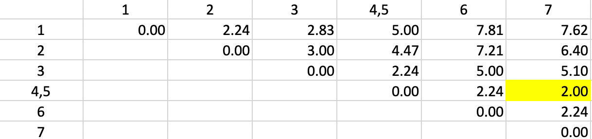
Figure 30: Single Linkage - Step 2

The dissimilarities between 4,5,7 and the other points are updated in Figure 31. But now we encounter a problem. There is a three-way tie in terms of the smallest value: 1-2, 4,5,7-3 and 4,5,7-6 all have a dissimilarity of 2.24, but only one can be picked to update the clusters. Ties can be handled by choosing one grouping at random. The algorithm behind the fastcluster implementation that is used by GeoDa selects the pair 1-2.

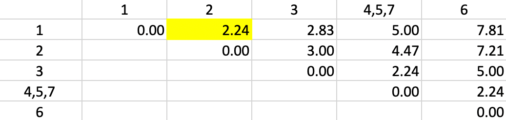
Figure 31: Single Linkage - Step 3

With the distances updated, we - not unsurprisingly - again find 2.24 as the shortest dissimilarity, tied for two pairs (in Figure 32). This time the algorithm adds 3 to the existing cluster 4,5,7.

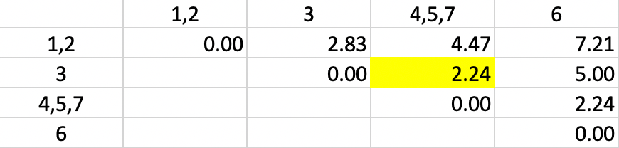
Figure 32: Single Linkage - Step 4

Finally, observation 6 is added to cluster 4,5,7,3 again for a dissimilarity of 2.24 (in Figure 33)

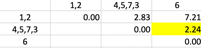
Figure 33: Single Linkage - Step 5

The end result is to merge the two clusters 1-2 and 4,5,7,3,6 into a single one, which ends the iterations (Figure 34).

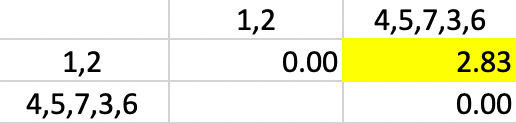
Figure 34: Single Linkage - Step 6

In GeoDa the consecutive grouping can be found from the categories assigned for each value of k and saved to the data table, as illustrated in Figure 35 (the cluster labels are arbitrary).⁸ The corresponding dendrogram is given in Figure 5.

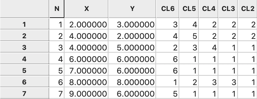
Figure 35: Single Linkage cluster categories saved in data table

Complete linkage worked example

The first step in the complete linkage algorithm is the same as in single linkage, since the dissimilarity between two single observations is unaffected by the criterion (the simple dissimilarity is also the minimum and the maximum). As before (Figure 29), observations 4 and 5 form the first cluster.

Next, we need to update the dissimilarities between the new cluster (4,5) and the other observations, by taking the largest dissimilarity between each observation and either 4 or 5. For example, for observation 1, we see from the dissimilarity matrix in Figure 2 that the respective values are 5.00 (1-4) and 5.83 (1-5). In contrast to the single linkage updating formula, we now assign 5.83 as the distance between 1 and the new cluster 4,5. We proceed in the same way for the other observations. The result is the updated dissimilarity matrix given in Figure 36. We encounter a tie situation for the smallest value (2.24) and pick 1,2 as the new cluster.

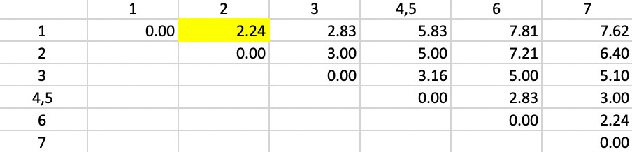
Figure 36: Complete Linkage - Step 2

The updated dissimilarity matrix is shown in Figure 37. Again, we take the largest dissimilarity between an observation (or cluster) and either 1 or 2. The smallest overall dissimilarity is still 2.24, now between 6 and 7, which form the next cluster.

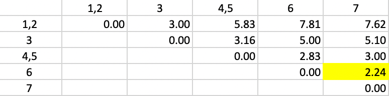
Figure 37: Complete Linkage - Step 3

The updated dissimilarity matrix is as in Figure 38. Now, the smallest dissimilarity is 3.00 (again a tie). We add 3 to 1,2 as the new cluster.

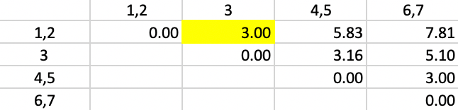
Figure 38: Complete Linkage - Step 4

This yields the updated dissimilarities as in Figure 39. The smallest dissimilarity is still 3.0, between 4,5 and 6,7. Those two clusters are grouped to yield the final result.

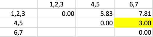
Figure 39: Complete Linkage - Step 5

In the end, we have two clusters, one consisting of 1,2,3, the other of 4,5,6,7, as shown in Figure 40.

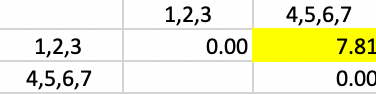
Figure 40: Complete Linkage - Step 6

In the same way as for single linkage, the consecutive grouping can be found in GeoDa from the categories assigned for each value of k and saved to the data table, as illustrated in Figure 41.

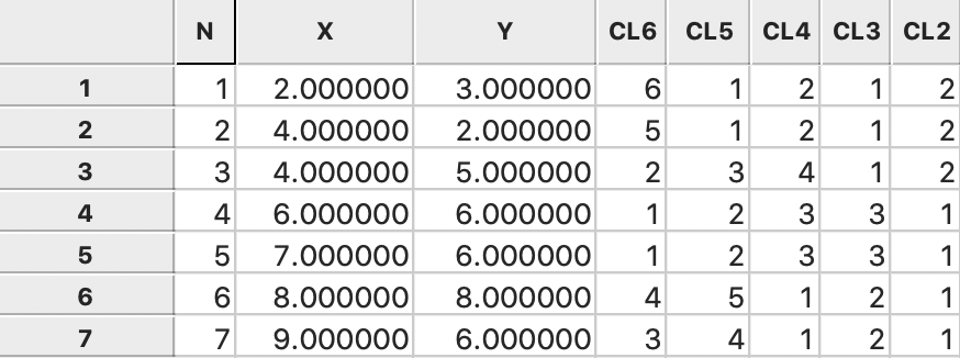
Figure 41: Complete linkage cluster categories saved in data table

Average linkage worked example

Average linkage begins like the other methods, by selecting 4,5 as the first cluster. As it turns out, in our example the updating formula for new clusters boils down to a simple average of the dissimilarities to both points/clusters, since all but the last merger is between balanced entities (e.g., 1 with 1 or 2 with 2). As a result, the weights attached to the respective distances, \(n_a / (n_a + n_b) = n_b / (n_a + n_b) = 1/2\).

For example, for observation 1, the new dissimilarity to 4,5 is (1/2) \(\times\) 5.00 + (1/2) \(\times\) 5.83 = 5.42 (due to some rounding) as shown in Figure 42. The other dissimilarities from/to 4,5 are updated in the same way. The smallest dissimilarity (a tie) in the updated table is 2.24 between 1 and 2, which are grouped into a new cluster.

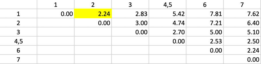
Figure 42: Average Linkage - Step 2

The new dissimilarities are shown in Figure 43, obtained as the average of the dissimilarities to 1 and 2 from the other points/clusters. In the new matrix, the smallest dissimilarity is again 2.24, between 6 and 7. They form the next cluster.

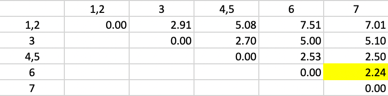
Figure 43: Average Linkage - Step 3

The updated dissimilarity matrix is given in Figure 44. The smallest dissimilarity is between clusters 4,5 and 6,7, which are combined in the next step.

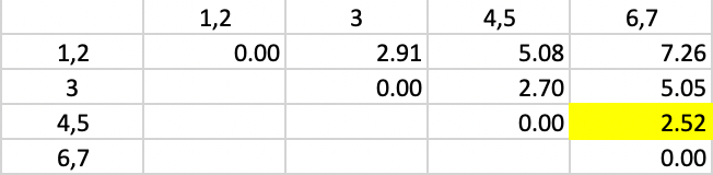
Figure 44: Average Linkage - Step 4

In the updated dissimilarity matrix of Figure 45, the minimum dissimilarity is between 3 and cluster 1,2. This yields the next to final grouping of 1,2,3 and 4,5,6,7.

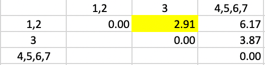
Figure 45: Average Linkage - Step 5

Only at this final stage is the computation of the averages somewhat more complex. Since the distance of 4,5,6,7 needs to be computed with respect to the merger of 1,2 and 3, the respective weights are 2/3 and 1/3. This yields the distance given in Figure 46.

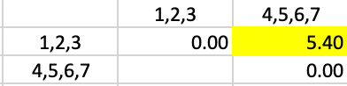
Figure 46: Average Linkage - Step 6

The consecutive steps in the nesting process can be found from the categories assigned for each value of k and saved to the GeoDa data table, as illustrated in Figure 47.

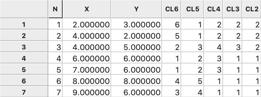
Figure 47: Average linkage cluster categories saved in data table

Ward’s method worked example

Ward’s method has the most complex updating formula of the four methods, involving not only the sum of the squared dissimilarity between every point and the components of the new cluster (\(d_{PA}^2\) and \(d_{PB}^2\)), with weights \((n_a + n_p)/(n_c + n_p)\) and \((n_b + n_p)/(n_c + n_p)\), but also subtracts the squared dissimilarity between the merging elements (\(d_{AB}^2\)), with weight \(n_p / (n_c + n_p)\). However, as is the case for the other methods, the updated dissimilarities can readily be computed from the matrix at the previous iteration.

The point of departure for Ward’s method is the matrix of squared Euclidian distances between the observations, as shown for our example in Figure 48. As before, the smallest value is between 4 and 5, with \(d_{4,5}^2 = 1.00\).

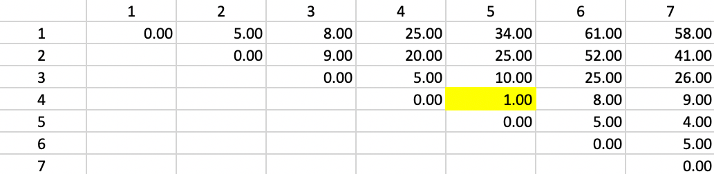
Figure 48: Ward Linkage - Step 1

Figure 49 shows the first updated squared distance matrix. Since the new squared distances pertain to single observations relative to a merged cluster of two single observations, \(n_a = n_b = n_p = 1\) and \(n_c = 2\). Therefore, the weights are 2/3 for \(d^2_{PA}\) and \(d^2_{PB}\) and 1/3 for \(d^2_{AB}\). For example, for the squared distance between 1 and 4,5, the updating formula becomes \((2/3) \times 25.00 + (2/3) \times 34.00 - (1/3) \times 1.0 = 39.00\). The other distances are computed in the same way. The squared distances that do not involve 4 or 5 are left unchanged.

The smallest squared distance in the matrix is between 1 and 2 with a value of 5.00. As before, there is a tie with 6 and 7, but the algorithm randomly picks 1,2. Hence, 1 and 2 are merged in the next step.

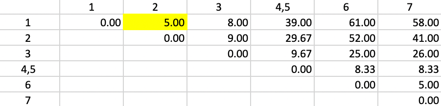
Figure 49: Ward Linkage - Step 2

The updated squared distances are shown in Figure 50. The values for the squared distances between 1,2 and 3, 6 and 7 use the same weights as in the previous step. For the squared distance between 1,2 and 4,5, \(n_p = 2\) and \(n_c = 2\), so that the weights become 3/4, 3/4 and 1/2. The smallest squared distance in the matrix is 5.00, between 6 and 7. Those two observations form the next cluster.

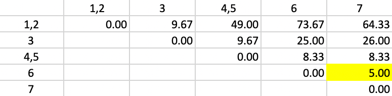
Figure 50: Ward Linkage - Step 3

The weights for the updating formula used in Figure 51 are the same as in the previous step. Now, there are two distances involving pairs of observations and one between a point and a pair. The smallest value in the updated matrix is 9.67, between 1,2 and 3. Subsequently, in the next step, 3 is added to the cluster consisting of 1 and 2.

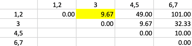
Figure 51: Ward Linkage - Step 4

The updates in Figure 52 involve squared distances between clusters of two observations (\(n_p = 2\)) and the new merger of two (\(n_a = 2\)) and one observation (\(n_b = 1\)), which gives \(n_c = 3\). The weights used in the update of 4,5 to 1,2,3 and 6,7 to 1,2,3 are therefore 4/5 for \(d^2_{PA}\), 3/5 for \(d^2_{PB}\) and 2/5 for \(d^2_{AB}\).

The smallest value in the matrix is 10.00 between 4,5, and 6,7, resulting in the merger of those two clusters in the next to final step.

Figure 52: Ward Linkage - Step 5

In the final matrix, the weights are 5/7 for \(d^2_{PA}\) and \(d^2_{PB}\), and 3/7 for \(d^2_{AB}\), yielding the squared distance of 93.90 between the two remaining clusters, as shown in Figure 53.

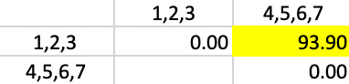
Figure 53: Ward Linkage - Step 6

As before, the consecutive steps in the nesting process are given in GeoDa by the categories assigned for each value of k and saved to the data table, as illustrated in Figure 54.

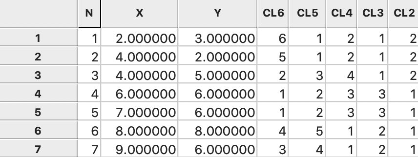
Figure 54: Ward linkage cluster categories saved in data table

References

Everitt, Brian S., Sabine Landau, Morven Leese, and Daniel Stahl. 2011. Cluster Analysis, 5th Edition. New York, NY: John Wiley.

Kaufman, L., and P. Rousseeuw. 2005. Finding Groups in Data: An Introduction to Cluster Analysis. New York, NY: John Wiley.

Müllner, Daniel. 2011. “Modern Hierarchical, Agglomerative Clustering Algorithms.” ArXiv:1109.2378[stat.ML]. http://arxiv.org/abs/1109.2378.

———. 2013. “fastcluster: Fast Hierarchical, Agglomerative Clustering Routines for R and Python.” Journal of Statistical Software 53 (9).

Ward, Joe H. 1963. “Hierarchical Grouping to Optimize an Objective Function.” Journal of the American Statistical Association 58: 236–44.

---

1. University of Chicago, Center for Spatial Data Science – anselin@uchicago.edu↩︎

2. Detailed proofs for all the properties are contained in Chapter 5 of Kaufman and Rousseeuw (2005).↩︎

3. To see that this holds, consider the situation when \(d_{PA} < d_{PB}\), i.e., \(A\) is the nearest neighbor to \(P\). As a result, the absolute value of \(d_{PA} - d_{PB}\) is \(d_{PB} - d_{PA}\). Then the expression becomes \((1/2) d_{PA} + (1/2) d_{PB} - (1/2) d_{PB} + (1/2) d_{PA} = d_{PA}\), the desired result.↩︎

4. Unlike what was the case for k-means, the center point does not play a role in single linkage clustering. Therefore, it is not shown in the Figure.↩︎

5. By convention, the diagonal dissimilarity for the newly merged cluster is set to zero.↩︎

6. See Kaufman and Rousseeuw (2005), Chapter 5, for detailed proofs.↩︎

7. The factor 2 is included to make sure the expression works when two single observations are merged. In such an instance, their centroid is their actual value and \(n_A + n_B = 2\). It does not matter in terms of the algorithm steps.↩︎

8. The data input to GeoDa is a csv file with the point IDs and X, Y coordinates.↩︎

GeoDa is maintained by lixun910. This page was generated by GitHub Pages using the Cayman theme by Jason Long.