Cluster Analysis (1)

K-Means Clustering

Introduction

We now move from reducing the dimensionality of the variables to reducing the number of observations, or clustering. In general terms, clustering methods group n observations into k clusters such that the intra-cluster similarity is maximized, and the between-cluster similarity is minimized. Equivalently, we can think of it as minimizing intra-cluster dissimilarity and maximizing between-cluster dissimilarity.

In other words, the goal of clustering methods is to achieve compact groups of similar observations that are separated as much as possible from the other groups.²

There are a very large number of clustering techniques and algorithms. They are standard tools of so-called unsupervised learning and constitute a core element in any machine learning toolbox. Classic texts include Hartigan (1975), Jain and Dubes (1988), Kaufman and Rousseeuw (2005), and Everitt et al. (2011). A fairly recent overview of methods can be found in Jain (2010), and an evaluation of k-means on a number of benchmark data sets is contained in Fränti and Sieranoja (2018). In addition, excellent treatments of some of the more technical aspects are contained in Chapter 14 of Hastie, Tibshirani, and Friedman (2009), Chapters 10 and 11 of Han, Kamber, and Pei (2012), and Chapter 10 of James et al. (2013), among others.

Clustering methods can be organized along a number of different dimensions. A common distinction is between partitioning methods, hierarchical methods, density-based methods and grid-based methods (see, e.g., Han, Kamber, and Pei 2012, 448–50). In addition, there are model-based approaches developed in the statistical literature, such as Gaussian mixture models (GMM) and Bayesian clusters.

In this and the next two chapters, we focus on the two most common approaches, namely partitioning methods and hierarchical methods. We do not cover the model-based techniques, since they are less compatible with an exploratory mindset (more precisely, they require a formal probabilistic model). We also restrict our discussion to exact clustering methods and do not consider fuzzy clustering (where an observation may belong to more than one cluster). In exact clustering, the clusters are both exhaustive and exclusive. This means that every observation must belong to one cluster, and only one cluster.

In the current chapter, we deal with k-means clustering, the most familiar example of a partitioning method. Hierarchical clustering is covered in the next chapter and more advanced techniques in a third.

To illustrate these methods, we will continue to use the Guerry data set on moral statistics in 1830 France, which comes pre-installed with GeoDa.

Objectives

• Understand the principles behind k-means clustering

• Know the requirements to carry out k-means clustering

• Interpret the characteristics of a cluster analysis

• Carry out a sensitivity analysis to various parameters

• Impose a bound on the clustering solutions

• Use an elbow plot to pick the best k

• Use the cluster categories as a variable

• Combine dimension reduction and cluster analysis

GeoDa functions covered

• Clusters > K Means
  • select variables
  • select k-means starting algorithms
  • select standardization methods
  • k-means characteristics
  • mapping the clusters
  • changing the cluster labels
  • saving the cluster classification
  • setting a minimum bound
• Explore > Conditional Plot > Box Plot
• Table > Aggregate
• Tools > Dissolve

K Means

Principle

Partitioning methods

A partitioning clustering method consists of assigning each observation to one out of \(k\) clusters. For each observation \(i\), this can be symbolized by an encoder C, such that \(C(i) = h\), where \(h\), the cluster indicator is an element from the set \(\{1, \dots, k\}\). The cluster labels (\(h\)) are meaningless, and could just as well be letters or other distinct symbols.³

The overall objective is to end up with a grouping that minimizes the dissimilarity within each cluster. Mathematically, we can think of an overall loss function that consists of summing the distances between all the pairs of observations (in general, any measure of dissimilarity): \[T = (1/2) \sum_{i = 1}^n \sum_{j = 1}^n d_{ij},\] where \(d_{ij}\) is some measure of dissimilarity, such as the Euclidean distance between the values at observations \(i\) and \(j\).⁴ The objective is then to find a grouping of the \(i\) into clusters \(h\) that minimizes this loss function, or, alternatively, maximizes the similarity (\(-T\)).

In any given cluster \(h\), we can separate out the distances from each of its members (\(i \in h\)) to all other observations between those that belong to the cluster (\(j \in h\)) and those that do not (\(j \notin h\)): \[T_{i \in h} = (1/2) [ \sum_{i \in h} \sum_{j \in h} d_{ij} + \sum_{i \in h} \sum_{j \notin h} d_{ij} ],\] and, for all the clusters, as: \[T = (1/2) (\sum_{h=1}^k [ \sum_{i \in h} \sum_{j \in h} d_{ij} + \sum_{i \in h} \sum_{j \notin h} d_{ij}]) = W + B,\] where the first term (\(W\)) is referred to as the within dissimilarity and the second (\(B\)) as the between dissimilarity. In other words, the total dissimilarity decomposes into one part due to what happens within each cluster and another part that pertains to the between cluster dissimilarities. \(W\) and \(B\) are complementary, so the lower \(W\), the higher \(B\), and vice versa. We can thus attempt to find an optimum by minimizing the within dissimilarity, \(W = (1/2) \sum_{h=1}^k \sum_{i \in h} \sum_{j \in h} d_{ij}\).

Partitioning methods differ in terms of how the dissimilarity \(d_{ij}\) is defined and how the term \(W\) is minimized. Complete enumeration of all the possible allocations is infeasible except for toy problems, and there is no analytical solution. The problem is NP-hard, so the solution has to be approached by means of a heuristic, as an iterative descent process. This is accomplished through an algorithm that changes the assignment of observations to clusters so as to improve the objective function at each step. All feasible approaches are based on what is called iterative greedy descent. A greedy algorithm is one that makes a locally optimal decision at each stage. It is therefore not guaranteed to end up in a global optimum, but may get stuck in a local one instead. The k-means method uses an iterative relocation heuristic as the optimization strategy (see Iterative relocation). First, we consider the associated dissimilarity measure more closely.

K-means objective function

The K-means algorithm is based on the squared Euclidean distance as the measure of dissimilarity: \[d_{ij}^2 = \sum_{v=1}^p (x_{iv} - x_{jv})^2 = ||x_i - x_j||^2,\] where we have changed our customary notation and now designate the number of variables/dimensions as \(p\) (since \(k\) is traditionally used to designate the number of clusters).

This gives the overall objective as finding the allocation \(C(i)\) of each observation \(i\) to a cluster \(h\) out of the \(k\) clusters so as to minimize the within-cluster similarity over all \(k\) clusters: \[\mbox{min}(W) = \mbox{min} (1/2) \sum_{h=1}^k \sum_{i \in h} \sum_{j \in h} ||x_i - x_j||^2,\] where, in general, \(x_i\) and \(x_j\) are \(p\)-dimensional vectors.

A little bit of algebra shows how this simplifies to minimizing the squared difference between the values of the observations in each cluster and the corresponding cluster mean (see the Appendix for details): \[\mbox{min}(W) = \mbox{min} \sum_{h=1}^k n_h \sum_{i \in h} (x_i - \bar{x}_h)^2.\]

In other words, minimizing the sum of (one half) of all squared distances is equivalent to minimizing the sum of squared deviations from the mean in each cluster, the within sum of squared errors.

Iterative relocation

The k-means algorithm is based on the principle of iterative relocation. In essence, this means that after an initial solution is established, subsequent moves (i.e., allocating observations to clusters) are made to improve the objective function. As mentioned, this is a greedy algorithm, that ensures that at each step the total across clusters of the within-cluster sums of squared errors (from the respective cluster means) is lowered. The algorithm stops when no improvement is possible. However, this does not ensure that a global optimum is achieved (for an early discussion, see Hartigan and Wong 1979). Therefore sensitivity analysis is essential. This is addressed by trying many different initial allocations (typically assigned randomly).

To illustrate the logic behind the algorithm, we consider a simple toy example of seven observations, as depicted in Figure 1. The full numerical details are given in the Appendix. The plot shows the location of the seven points in two-dimensional \(X-Y\) space, with the center (the mean of \(X\) and the mean of \(Y\)) shown in a lighter color (note that the center is not one of the observations). The objective is to group the seven points into two clusters.

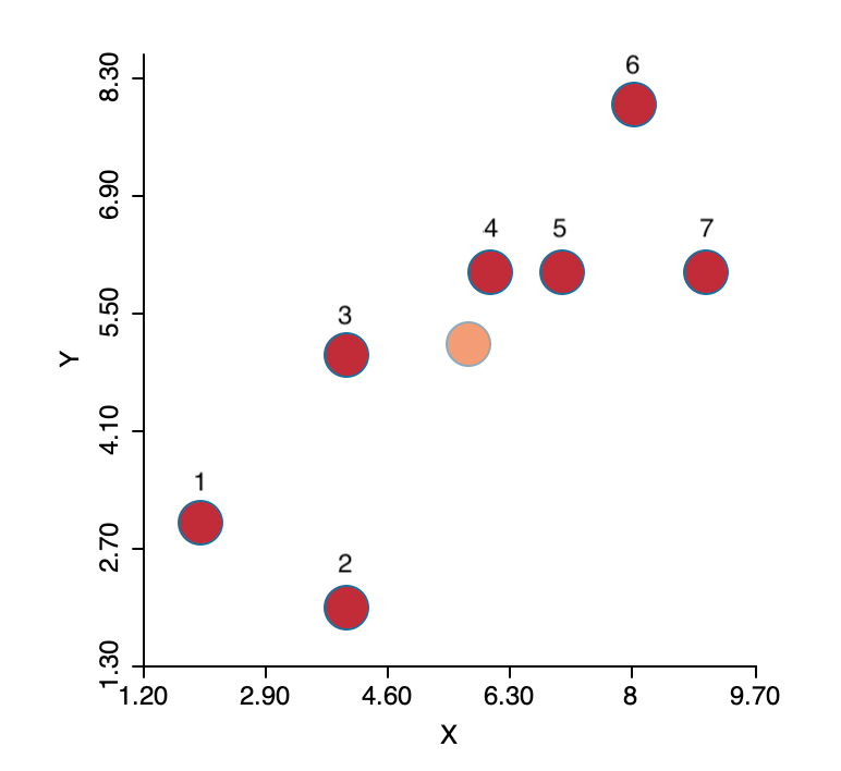
Figure 1: K-means toy example

The initial step of the algorithm is to randomly pick two seeds, one for each cluster. The seeds are actual observations, not some other random location. In our example, we selected observations 4 and 7, shown by the lighter color in the upper left panel of Figure 2. The other observations are allocated to the cluster whose seed they are closest to. We see that the green cluster has one other observation (6, in dark green), and the blue cluster four more (in dark blue). This is the initial layout, shown in the top right panel of the figure: two observations in one cluster and five in the other.

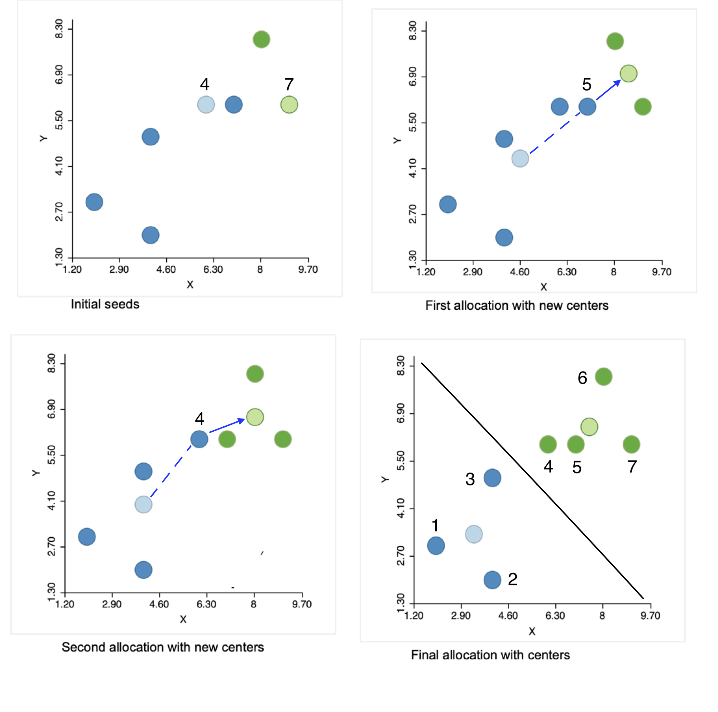
Figure 2: Steps in the k-means algorithm

Next, we compute the center for each cluster, i.e., the mean of each coordinate, shown in the figure in the lighter color. Note that from this point on, the center is no longer one of the observations (or only by coincidence).

The first real step of the algorithm allocates observations to the cluster center they are closest to. In the top right panel, we see that point 5 from the original blue cluster is closer to the new center for the green cluster than to the new center for the blue cluster. Consequently, it moves to join the green cluster, which now consists of three observations (in the lower left panel).

We repeat the process with the new centers in the lower left panel and again find point 4 from the blue cluster closer to the updated center for the green cluster, so it joins the latter. This yields one cluster of four (green) observations (closest to the center in the upper right panel) and one of three (blue) observations.

This process is repeated until no more improvement is possible. In our example, we are done after the two steps, since all observations are closest to their center. The lower-right panel in the figure shows the final allocation with associated centers.

This solution corresponds to the allocation that would result from a Voronoi diagram or Thiessen polygon around the cluster centers. All observations are closer to their center than to any other center. This is indicated by the black line in the graph, which is perpendicular at the midpoint to an imaginary line connecting the two centers and separates the area into two compact regions.

The choice of K

A key element in the k-means method is the choice of the number of clusters, k. Typically, several values for k are considered, and the resulting clusters are then compared in terms of the objective function.

Since the total sum of squared errors (SSE) equals the sum of the within-group SSE and the total between-group SSE, a common criterion is to assess the ratio of the total between-group sum of squares (BSS) to the total sum of squares (TSS), i.e., BSS/TSS. A higher value for this ratio suggests a better separation of the clusters. However, since this ratio increases with k, the selection of a best k is not straightforward. Several ad hoc rules have been suggested, but none is totally satisfactory.

One useful approach is to plot the objective function against increasing values of k. This could be either the within sum of squares (WSS), a decreasing function with k, or the ratio BSS/TSS, a value that increases with k. The goal of a so-called elbow plot is to find a kink in the progression of the objective function against the value of k. The rationale behind this is that as long as the optimal number of clusters has not been reached, the improvement in the objective should be substantial, but as soon as the optimal k has been exceeded, the curve flattens out. This is somewhat subjective and often not that easy to interpret in practice. GeoDa’s functionality does not include an elbow plot, but all the information regarding the objective functions needed to create such a plot is provided in the output.

A more formal approach is the so-called Gap statistic of Tibshirani, Walther, and Hastie (2001), which employs the difference between the log of the WSS and the log of the WSS of a uniformly randomly generated reference distribution (uniform over a hypercube that contains the data) to construct a test for the optimal k. Since this approach is computationally quite demanding, we do not consider it here.

K-means algorithms

The earliest solution of the k-means problem is commonly attributed to Lloyd (1982) and referred to as Lloyd’s algorithm (the algorithm was first contained in a Bell Labs technical report by Lloyd from 1957). While the progression of the iterative relocation is fairly straightforward, the choice of the initial starting point is not.⁵

Typically, the assignment of the first set of k cluster centers is obtained by uniform random sampling k distinct observations from the full set of n observations. In other words, each observation has the same probability of being selected.

The standard approach is to try several random assignments and start with the one that gives the best value for the objective function (e.g., the smallest WSS). This is one of the two approaches implemented in GeoDa. In order to ensure replicability, it is important to set a seed value for the random number generator. Also, to further assess the sensitivity of the result to the starting point, different seeds should be tried (as well as a different number of initial solutions). GeoDa implements this approach by leveraging the functionality contained in the C Clustering Library (Hoon, Imoto, and Miyano 2017).

A second approach uses a careful consideration of initial seeds, following the procedure outlined in Arthur and Vassilvitskii (2007), commonly referred to as k-means++. The rationale behind k-means++ is that rather than sampling uniformly from the n observations, the probability of selecting a new cluster seed is changed in function of the distance to the nearest existing seed. Starting with a uniformly random selection of the first seed, say \(c_1\), the probabilities for the remaining observations are computed as: \[p_{j \neq c_1} = \frac{d_{jc_1}^2}{\sum_{j \neq c_1} d_{jc_1}^2 }.\] In other words, the probability is no longer uniform, but changes with the squared distance to the existing seed: the smaller the distance, the smaller the probability. This is referred to by Arthur and Vassilvitskii (2007) as the squared distance (\(d^2\)) weighting.

The weighting increases the chance that the next seed is further away from the existing seeds, providing a better coverage over the support of the sample points. Once the second seed is selected, the probabilities are updated in function of the new distances to the closest seed, and the process continues until all k seeds are picked.

While generally being faster and resulting in a superior solution in small to medium sized data sets, this method does not scale well (as it requires k passes through the whole data set to recompute the distances and the updated probabilities). Note that a choice of a large number of random initial allocations may yield a better outcome than the application of k-means++, at the expense of a somewhat longer execution time.

Implementation

We invoke the k-means functionality from the same Clusters toolbar icon as we have seen previously for dimension reduction. It is part of the second subset of functionality, which includes several classic and more advanced (non-spatial) clustering techniques, as shown in Figure 3. From the menu, it is selected as Clusters > K Means.

Figure 3: K Means Option

This brings up the K Means Clustering Settings dialog, shown in Figure 4, the main interface through which variables are chosen, options selected, and summary results are provided.

Variable Settings panel

We select the variables and set the parameters for the K Means cluster analysis through the options in the left hand panel of the interface. We choose the same six variables as in the previous chapter: Crm_prs, Crm_prp, Litercy, Donatns, Infants, and Suicids. These variables appear highlighted in the Select Variables panel.

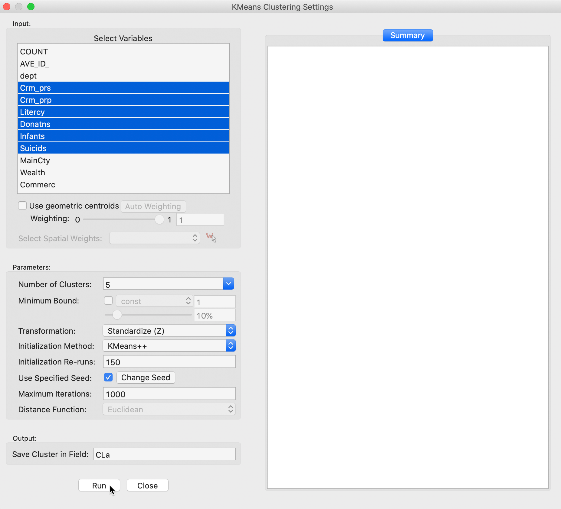
Figure 4: K Means variable selection

The next option is to select the Number of Clusters. The initial setting is blank. One can either choose a value from the drop-down list, or enter an integer value directly.⁶ In our example, we set the number of clusters to 5.

A default option is to use the variables in standardized form, i.e., in standard deviational units, expressed with Transformation set to Standardize (Z).⁷

The default algorithm is KMeans++ with initialization re-runs set to 150 and maximal iterations to 1000. The seed is the global random number seed set for GeoDa, which can be changed by means of the Use specified seed option. Finally, the default Distance Function is Euclidean. For k-means, this is the only option available, since it is the basis for the objective function.

The cluster classification will be saved in the variable specified in the Save Cluster in Field box. The default of CL is likely not very useful if several options will be explored. In our first example, we set the variable name to CLa.

Cluster results

After pressing Run, and keeping all the settings as above, a cluster map is created as a new view and the characteristics of the cluster are listed in the Summary panel.

The cluster map in Figure 5 reveals quite evenly balanced clusters, with 22, 19, 18, 16 and 10 members respectively. Keep in mind that the clusters are based on attribute similarity and they do not respect contiguity or compactness (we will examine spatially constrained clustering in a later chapter).

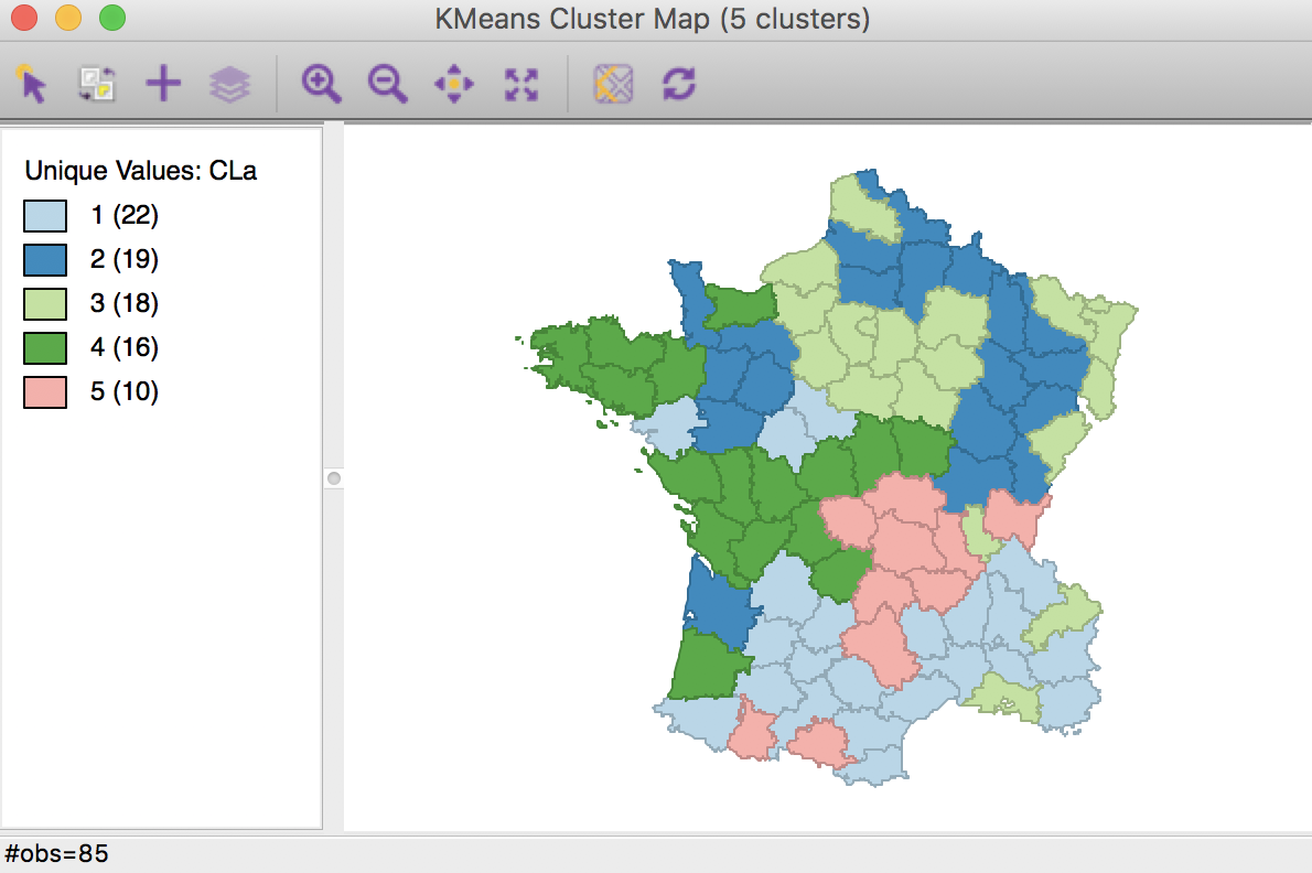
Figure 5: K Means cluster map (k=5)

The cluster characteristics are listed in the Summary panel, shown in Figure 6. This lists, for each cluster, the method (KMeans), the value of k (here, 5), as well as the parameters specified (i.e., the initialization methods, number of initialization re-runs, the maximum iterations, transformation, and distance function).

Next follows a table with the values of the cluster centers for each of the variables involved in the clustering algorithm. Note that while the algorithm uses standardized values (with the Standardize option on), the results are presented in the original units. This allows for a comparison of the cluster means to the overall mean of the variable. In our example, the overall means are 19,961 for Crm_prs, 7,881 for Crm_prp, 39.1 for Litercy, 6,723 for Donatns, 18,983 for Infants, and 36,517 for Suicids. The interpretation is not always straightforward due to the complex interplay among the variables. In our example, none of the clusters have a mean that is superior to the national average for all variables. Cluster 3 is below the national mean for all but one variable (litercy). In a typical application, a close examination of these profiles should be the basis for any kind of meaningful characterization of the clusters (e.g., as in a socio-demographic profile).

Finally, a number of summary measures are provided to assess the overall quality of the cluster results. The total sum of squares is listed (504), as well as the within-cluster sum of squares for each of the clusters. The absolute values of these results are not of great interest, but their relative magnitudes matter. For example, we can see that the similarity within cluster 3 (18 observations) is more than twice as good (less than half) as that in clusters 4 and 5.

Finally, these statistics are summarized as the total within-cluster sum of squares (253.277), the total between-cluster sum of squares (the difference between TSS and WSS, 250.723), and the ratio of between-cluster to total sum of squares. In our initial example, the latter is 0.497467.

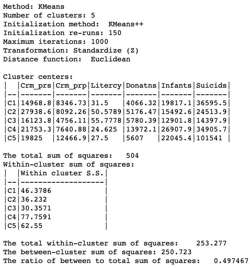
Figure 6: K Means cluster characteristics (k=5)

Adjusting cluster labels

The cluster labels (and colors in the map) are arbitrary and can be changed in the cluster map, using the same technique we saw earlier for unique value maps (in fact, the cluster maps are a special case of unique value maps). For example, if we wanted to switch category 4 with 3 and the corresponding colors, we would move the light green rectangle in the legend with label 4 up to the third spot in the legend, as shown in Figure 7.

Figure 7: Change cluster labels

Once we release the cursor, an updated cluster map is produced, with the categories (and colors) for 3 and 4 switched, as in Figure 8.

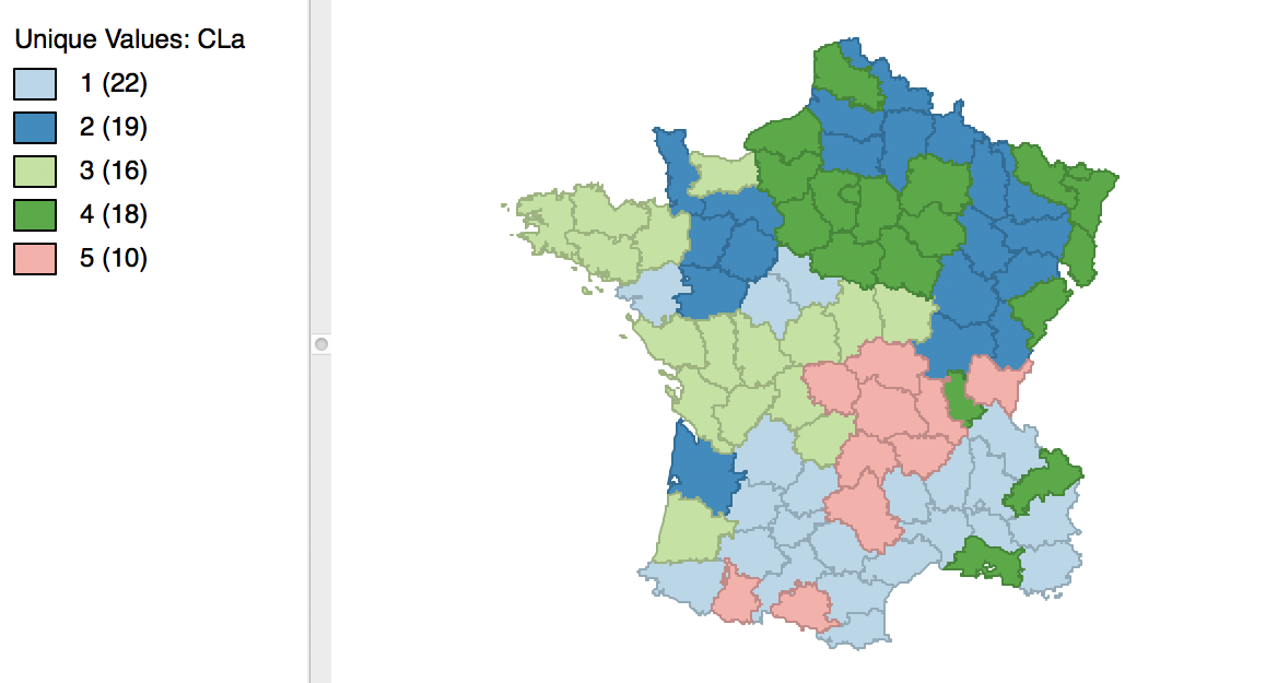
Figure 8: Relabeled cluster map

Cluster variables

As the clusters are computed, a new categorical variable is added to the data table (the variable name is specified in the Save Cluster in Field option). It contains the assignment of each observation to one of the clusters as an integer variable. However, this is not automatically updated when we change the labels, as we did in the example above.

In order to save the updated classification, we can still use the generic Save Categories option available in any map view (right click in the map). After specifying a variable name (e.g., cat_a), we can see both the original categorical variable and the new classification in the data table.

In the table, shown in Figure 9, wherever CLa (the original classification) is 3, the new classification (cat_a) is 4. As always, the new variables do not become permanent additions until the table is saved.

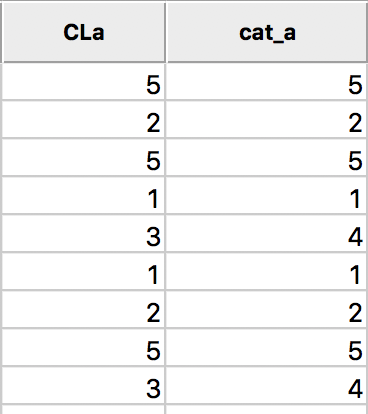
Figure 9: Cluster categories in table

Saving the cluster results

The summary results listed in the Summary panel can be saved to a text file. Right clicking on the panel to brings up a dialog with a Save option, as in Figure 10. Selecting this and specifying a file name for the results will provide a permanent record of the analysis.

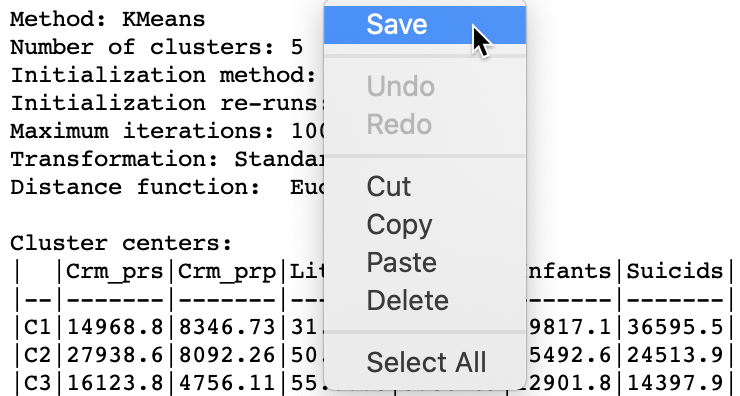
Figure 10: Saving summary results to a text file

Options and sensitivity analysis

The k-means algorithm depends crucially on its initialization and on the various parameters specified. It is important to assess the sensitivity of the results to the starting point and other parameters and settings. We consider a few of these next.

Changing the number of k-means++ initial runs

The default number of initial re-runs for the k-means++ algorithm is 150. Sometimes, this is not sufficient to guarantee the best possible result (e.g., in terms of the ratio of between to total sum of squares). Recall that k-means++ is simply a different way to have random initialization, so it also offers no guarantees with respect to the optimality of the starting point.

We can change the number of initial runs to obtain a starting point from the k-means++ algorithm in the Initialization Re-runs dialog, as illustrated in Figure 11 for a value of 1000 iterations.

Figure 11: K-means++ initialization re-runs

The result is slightly different from what we obtained for the default setting. As shown in Figure 12, the first category now has 23 elements, and the second 18. The other groupings remain the same.

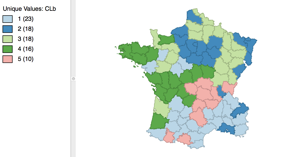
Figure 12: Cluster map for 1000 initial re-runs

The revised initialization results in a slight improvement of the sum of squares ratio, changing from 0.497467 to 0.497772, as shown in Figure 13.

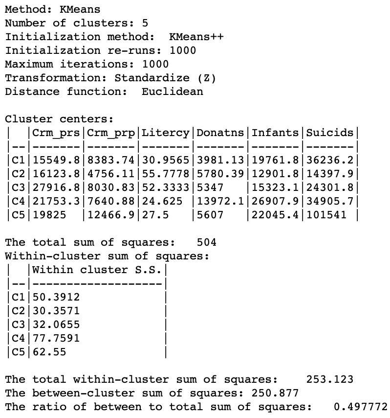
Figure 13: Cluster characteristics for 1000 initial reruns

Random initialization

The alternative to the Kmeans++ initialization is to select the traditional random initialization with uniform probabilities across the observations. This is accomplished by choosing Random as the Initialization Method, as shown in Figure 14. We keep the number of initialization re-runs to the default value of 150 and save the result in the variable CLr.

Figure 14: Random initialization

The result is identical to what we obtained for K-means++ with 1000 initialization re-runs, with the cluster map as in Figure 12 and the cluster summary as in Figure 13. However, if we had run the random initialization with much fewer runs (e.g., 10), the results would be inferior to what we obtained before. This highlights the effect of the starting values on the ultimate result.

Selecting a different standardization

The objective function for k-means clustering is sensitive to the scale in which the variables are expressed. When these scales are very different (e.g., one variable is as a percentage and another is expressed as thousands of dollars), standardization converts the observations to more comparable magnitudes. As a result, the squared differences (or squared difference from the cluster mean) become more or less comparable across variables. More specifically, this avoids that variables that show a large variance dominate the objective function.

The most common standardization is the so-called z-standardization, where the original value is centered around zero (by subtracting the mean) and rescaled to have a variance of one (by dividing by the standard deviation). However, this is by no means the only way to correct for the effect of different spreads among the variables. Some other approaches, which may be more robust to the effect of outliers (on the estimates of mean and variance used in the standardization) are the MAD, mentioned in the context of PCA, as well as range standardization. The latter is often recommended for cluster excercises (e.g., Everitt et al. 2011). It rescales each variable such that its minimum is zero and its maximum becomes one by subtracting the minimum and dividing by the range.

We assess the effect of such a standardization on the k-means result by selecting the associated option, as in Figure 15. We leave all the other options to the default setting.

Figure 15: Range Standardization

The resulting clusters are depicted in Figure 16. Compared to the standard result in Figure 5, the spatial layout of cluster members is quite different. Two of the clusters are larger (1 and 2 with 27 and 20 elements) and two others smaller (3 and 4 with 17 and 11). Cluster 5 has the same number of members as in the original solution, but only half the observations are in common.

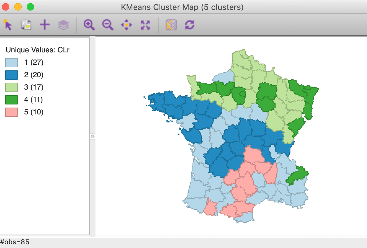
Figure 16: Cluster map for range standardization

The difference between the two solutions is also highlighted by the cluster summary measures, shown in Figure 17. Clusters 3, 4 and 5 are almost equally compact and the overall BSS/TSS ratio is the highest achieved so far, at 0.537.

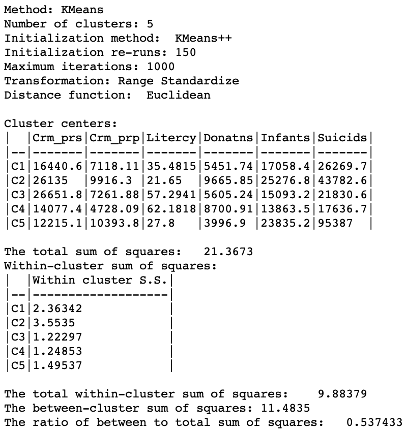
Figure 17: Cluster characteristics for range standardization

This again highlights the need to carry out sensitivity analysis and not take the default standardization as the only available option. Depending on the relative ranges and variances of the variables under consideration, one standardization may achieve a better grouping than another. Also, in some circumstances, when the variables are already on similar scales, standardization is not necessary.

Setting a minimum bound

It is also possible to constrain the k-means clustering by imposing a minimum value for a spatially extensive variable, such as a total population. This ensures that the clusters meet a minimum size for that variable. For example, in studies of socio-economic determinants of health, we may want to group similar census tracts into neighborhoods. But if we are concerned with rare diseases, privacy concerns often require a minimum size for the population at risk. By setting a minimum bound on the population variable, we avoid creating clusters that are too small.

The minimum bound is set in the variable settings dialog by checking the box next to Minimum Bound, as in Figure 18. This variable does not have to be part of the variables used in the clustering exercise. In fact, it should be a relevant size variable (so-called spatially extensive variable), such as total population or total number of establishments, unrelated to the multivariate dimensions involved in the clusters.

In our example, we select the variable Pop1831 to set the constraint. Note that we specify a bound of 16% (or 5179) rather than the default 10%. This is because the standard k-means solution satisfies the default constraint already, so that no actual bounding is carried out. Also, any percentage higher than 16 fails to yield a cluster solution that meets the population requirement.

Figure 18: Setting a minimum bound

With the cluster size at 5 and all other options back to their default value, (specifically, with 150 kmeans++ initialization runs) we obtain the cluster result shown in the map in Figure 19. The categories have been re-ordered to show a similar color scheme to the unconstrained map in Figure 5 (using CLc as the cluster variable).

Figure 19: Cluster map with minimum bound constraint

Relative to the unconstrained map, we find that three clusters have increased in size (1 to 22, 2 to 19 and 4 to 16) and two shrank (3 to 19 and 5 to 10). In addition, the configuration of the clusters changed slightly as well, with cluster 5 the most affected.

The cluster characteristics show a slight deterioriation of our summary criterion, to a value of 0.484033 (compared to 0.497772), as shown in Figure 20. This is the price to pay to satisfy the minimum population constraint. However, the effect on the individual clusters is mixed, with clusters 2 and 5 having a much worse WSS, whereas 1, 3 and 4 actually achieve a smaller WSS relative to the unconstrained version. This illustrates the complex trade-offs involved between the cases where the constraint has to be enforced compared to where it is already satisfied.

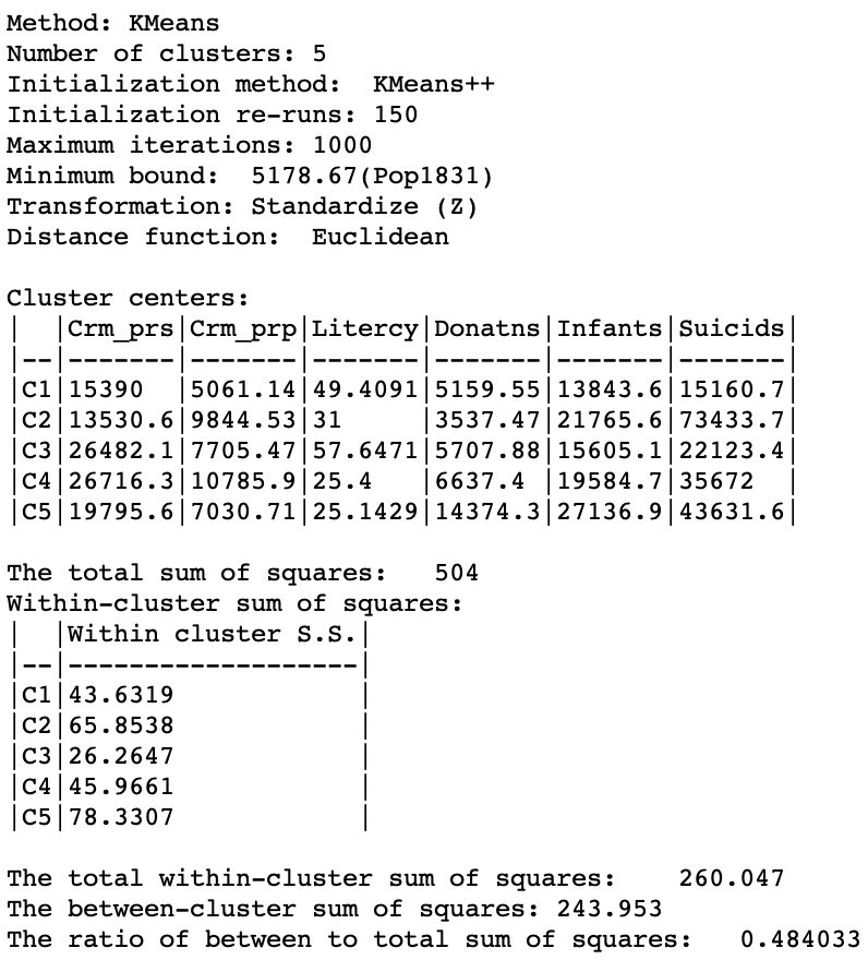
Figure 20: Cluster characteristics with minimum bound

Elbow plot

We now illustrate the use of an elbow plot to assess the best value for k. This plot is not included in the GeoDa functionality, but it is easy to construct from the output of a cluster analysis.

The results for runs of k-means with all the default settings are given in Figure 21, for k ranging from 1 through 12. As the number of clusters increases, the resulting groupings become less and less informative and tend to yield several singleton clusters (with only one observation). Both WSS and BSS/TSS are listed, with the associated change as the value of k increases.

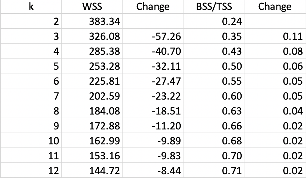
Figure 21: Cluster characteristics for increasing values of k

The actual elbow plots are given in Figure 22. There are two versions of this plot, one showing the decrease in WSS as k increases (left panel of the Figure), the other illustrating the increase in the ratio BST/SST with k (right panel). Unlike the usual textbook examples, in our case these graphs are not easy to interpret, still showing an albeit smaller improvement for \(k > 10\), which is not a practical number of clusters for only 85 observations. It does seem that a good value for k would be in the range 5-8, although this is by no means a hard and fast conclusion.

This example illustrates the difficuly of deciding on the best k in practice. Considerations other than those offered by the simple elbow plot should be taken into account, such as how to interpret the groupings that result from the cluster analysis and whether the clusters are reasonably balanced. In some sense this is both an art and a science and it takes practice as well as familiarity with the substantive research questions to obtain a good insight into the trade-offs involved.

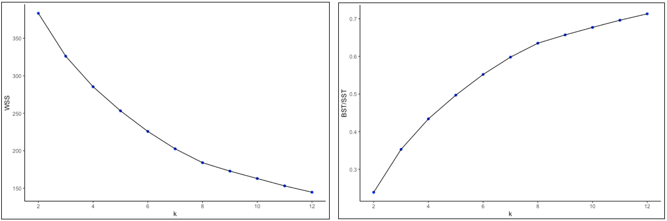
Figure 22: Elbow plots

Cluster Categories as Variables

Once added to the data table, the cluster categories can be visualized like any other integer variable. We already saw their use in the unique values map that is provided with the standard output. Two other particularly useful applications are as a conditioning variable in a conditional plot and as a variable to guide aggregation of observations to the cluster level.

Conditional plots

A particularly useful conditional plot is a conditional box plot, in which the distribution of a variable can be shown for each cluster. This supplements the summary characteristics of each cluster provided in the standard output, where only the mean is shown for each cluster category.

The conditional box plot is invoked as Explore > Conditional Plot > Box Plot, or from the conditional plots icon on the toolbar, as in Figure 23.

Figure 23: Conditional box plot option

For this particular application, it is most effective to only condition on one dimension, either horizontal or vertical. In the dialog shown in Figure 24, we selected the cluster variable CLa as the horizontal axis. We also selected the empty category for the vertical axis (this ensures that conditioning only happens in the horizontal dimension), and chose Litercy as the variable.

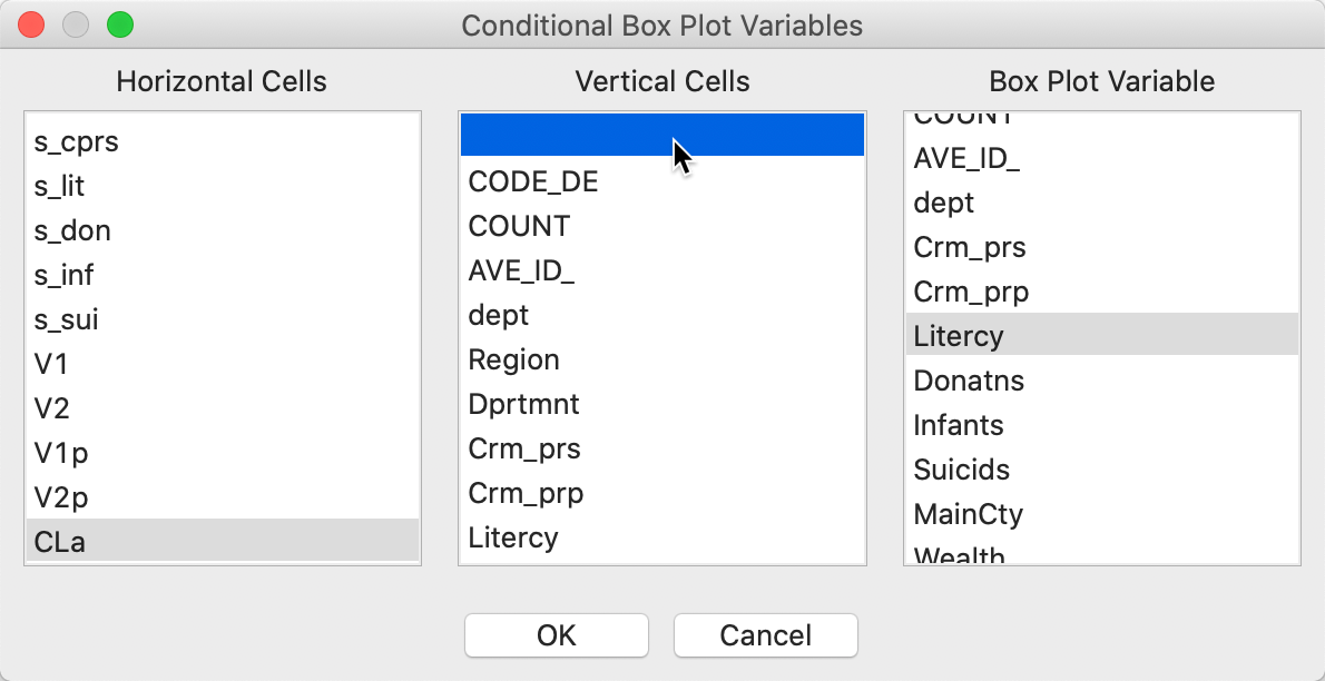
Figure 24: Conditional box plot variable selection

The first plot that results is not very useful, since it takes a quantile distribution as the default for the horizontal axis. By right clicking, the options are brought up and we select Horizontal Bins Breaks > Unique Values. The result is as in Figure 25.

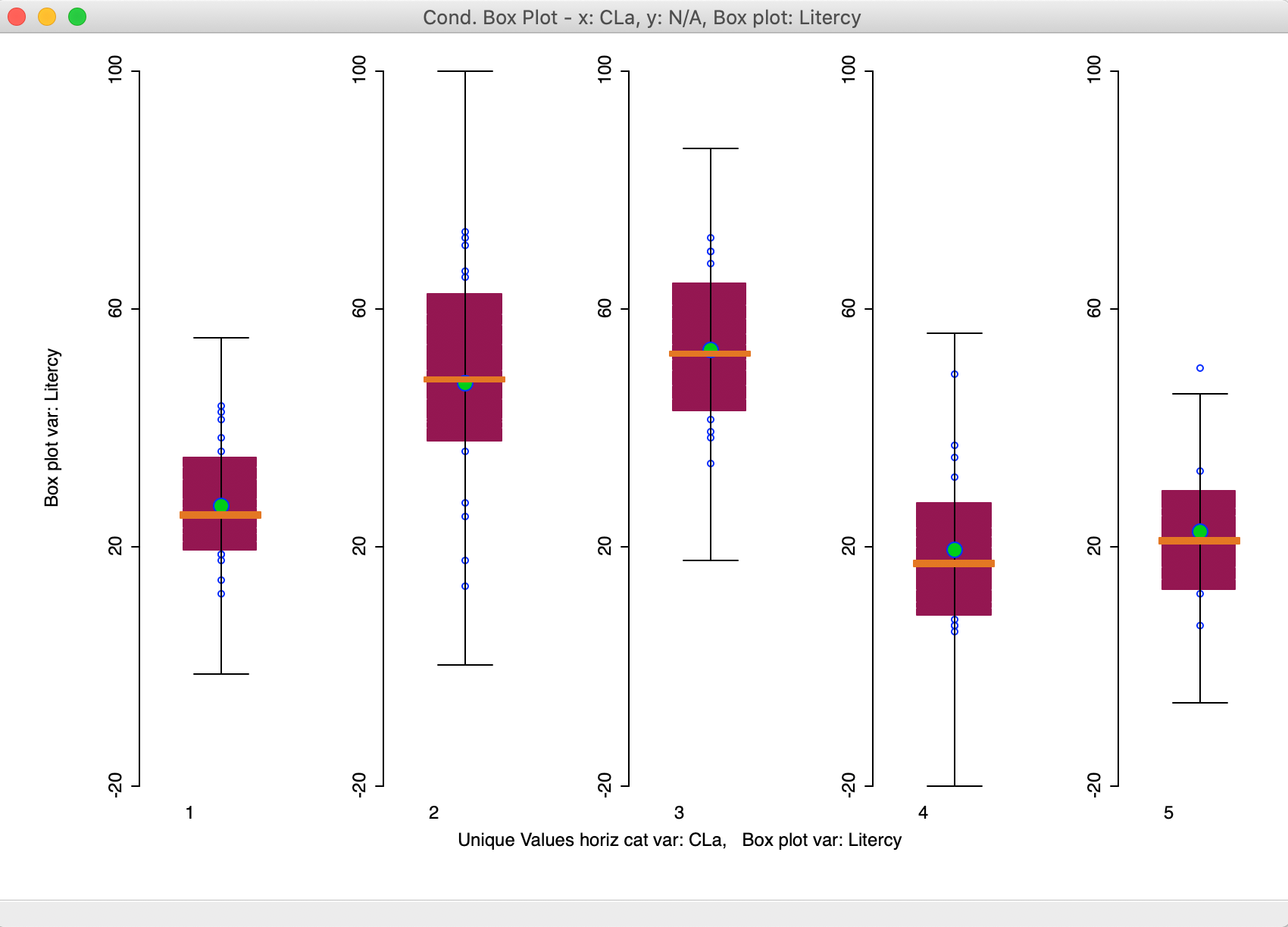
Figure 25: Conditional box plot for literacy

The box plots use the same scale, so that comparisons are easy to make. Note that even though the box plot fences are drawn, the actual range of the distribution in each cluster does not necessarily reach that far. In our example, the values for clusters 1-3 are well within these bounds. Only for cluster 5 do we observe an outlier.

The plot clearly shows how the median value is much higher for clusters 2 and 3 relative to the others. It also shows little overlap of the interquartile range between the two groups (2 and 3, relative to 1-4-5). Conditional box plots can be a useful aide in the characterization of the different clusters in that they provide more than just a summary measure, such as a mean or median, but portray the whole distribution.

Aggregation by cluster

With the clusters at hand, as defined for each observation by the category in the cluster field, we can now compute aggregate values for the new clusters and even create new layers for the dissolved units. We illustrate this as a quick check on the population totals we imposed in the bounded cluster procedure.

There are two different ways to proceed. In one, we only create a new table, in the other, we end up with a new layers that has the original units spatially dissolved into the new clusters.

The simple aggregation is invoked from the Table as an option by right-clicking. This brings up the list of options, from which we select Aggregate, as in Figure 26.

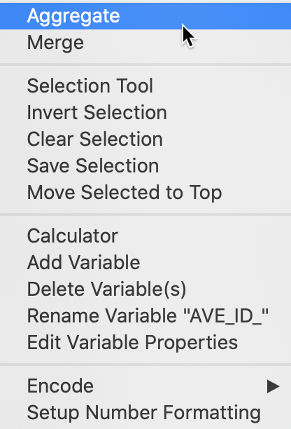
Figure 26: Table Aggregate option

The following dialog, shown in Figure 27, provides the specific aggregation method, i.e., count, average, max, min, or Sum, the key on which to aggregate and a selection of variable to aggregate. In our example, we use the cluster field key, e.g., CLc (from the bounded clustering solution) and select only the population variable Pop1831, which we will sum over the departments that make up each cluster. This can be readily extended to multiple variables, as well as to different summary measures, such as the average.⁸

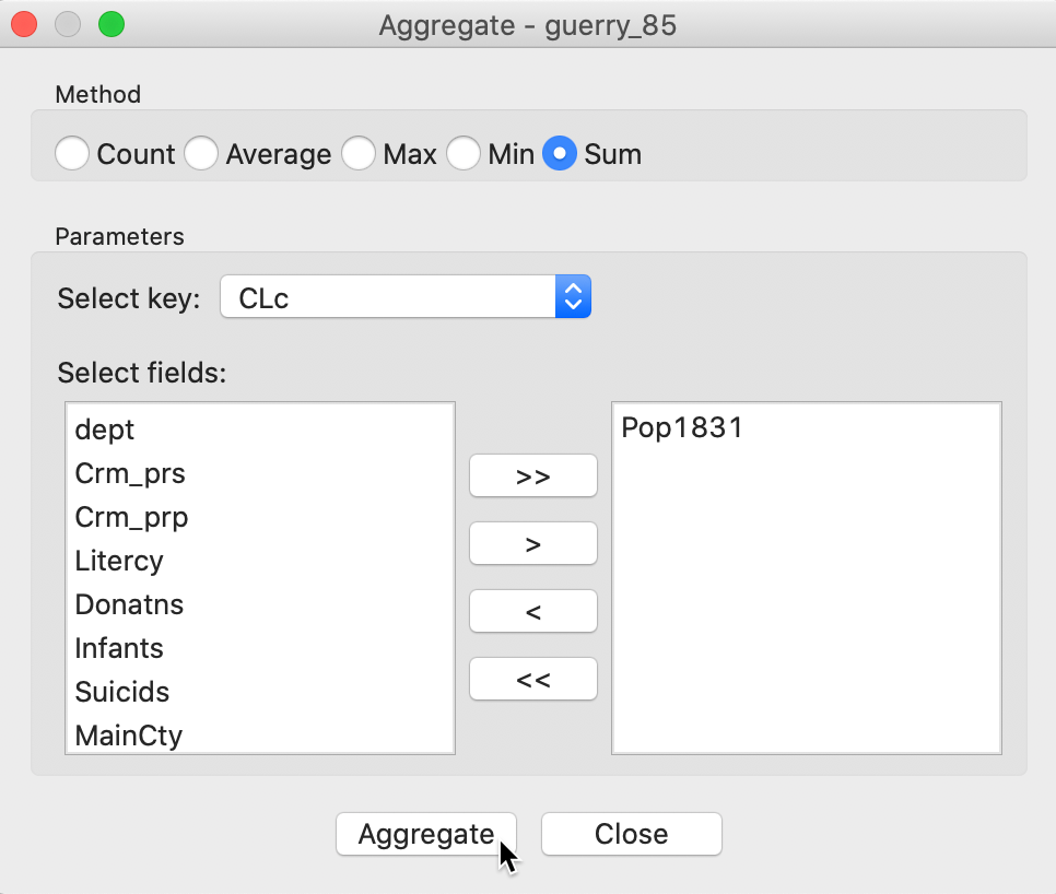
Figure 27: Aggregation of total population by cluster

Pressing the Aggregate key brings up a dialog to select the file in which the new results will be saved. For example, we can select a dbf format and specify the file name. The contents of the new file are given in Figure 28, with the total population for each cluster. Clearly, each cluster meets the minimum requirement of 5179 that was specified.

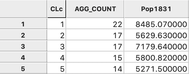
Figure 28: Total population by cluster

The same procedure can be used to create new values for any variable, aggregated to the new cluster scale. Note that since most variables in the Guerry data set are ratios, a simple sum would not be appropriate.

A second way to create new aggregate spatial units is to invoke the Dissolve functionality from the Tools menu as in Figure 29. This will aggregate the variables in the same way as for the table, but also create a new spatial layer that dissolves the original units into their new aggregate clusters.

Figure 29: Dissolve function

The next interface is the same as for the aggregate functionality, shown in Figure 27. We again select CLc as the key to aggregate the spatial units and specify Pop1831 as the variable to be summed into the new units. After saving the new layer, we can bring it back into GeoDa and create a unique values map of the population totals, as in Figure 30.⁹ The table associated with this layer is identical to the one shown in Figure 28.

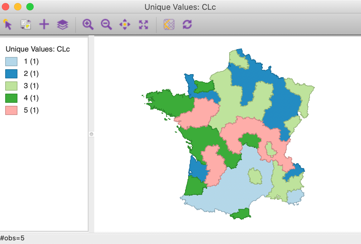
Figure 30: Map of clusters with population totals

Clustering with Dimension Reduction

In practice, it is often more effective to carry out a clustering exercise after dimension reduction, instead of using the full set of variables. This is typically based on principal components, but can equally be computed from the MDS coordinates. Both approaches are illustrated below.

PCA

Instead of specifying all six variables, we carry out k-means clustering for the first two principal components, say the variables PC1 and PC2. Since the principal components are already standardized, we can set that option to Raw. The results for k=5 are shown in Figure 31, with the coordinates in a two-dimensional principal component scatter plot on the left, and the associated cluster map on the right. The clusters appear as clear regions in the scatter plot, highlighting the (multivariate) similarity among those observations in the same cluster.¹⁰

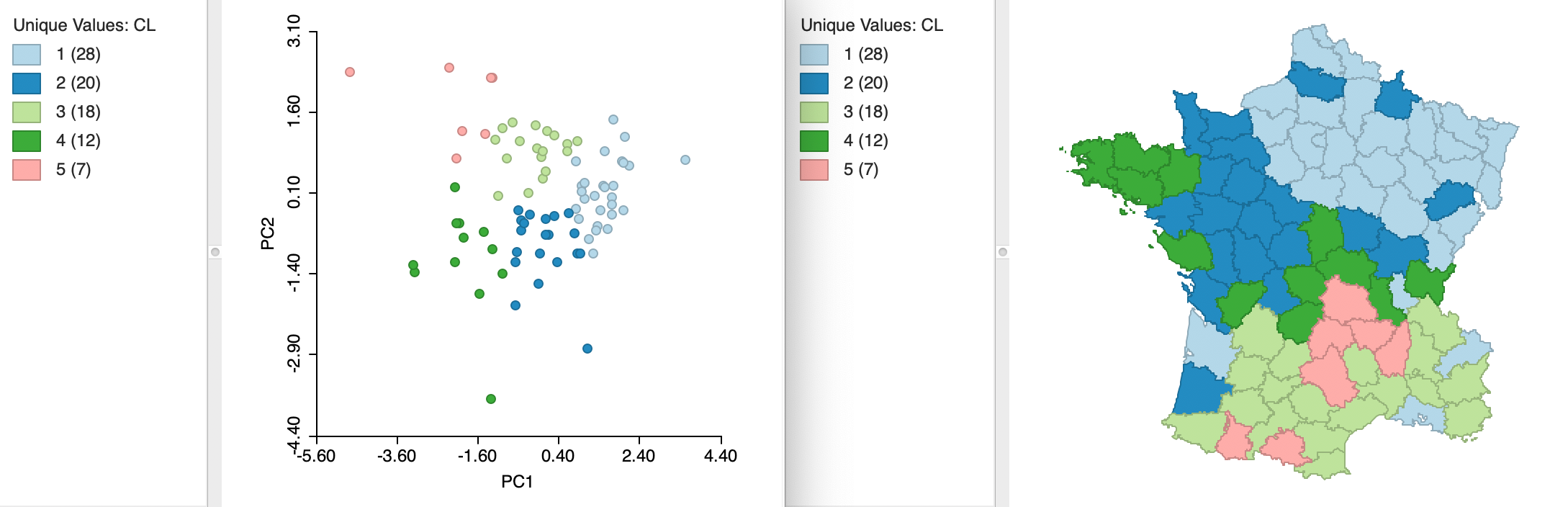
Figure 31: PCA plot and cluster map

A summary with the cluster centers, the associated WSS and summary statistics is given in Figure 32. Strikingly, the between sum of squares to total sum of squares ratio is 0.755, by far the best cluster separation obtained for k=5 (and even better than the six-variable result for k=12). This illustrates the potential gain in efficiency obtained by reducing the full six variable dimensions to the principal components, which effectively summarize the multivariate characteristics of the data.

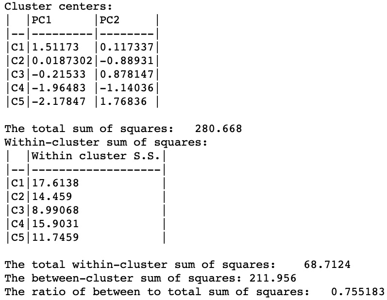
Figure 32: PCA cluster summary

MDS

The same principle can be applied to the coordinates obtained from multidimensional scaling. While this is less used in practice, it is in fact equivalent to using principal components. We have already seen that for classic metric scaling the two-dimensional plots of the two approaches are equivalent, except for flipping the axes. This can also be seen from the results for k=5 shown in Figure 33. The variables used in the clustering exercise are the MDS coordinates V1 and V2 (again, with the standardization option set to Raw). The clusters are identical to those obtained for the first two principal components. The scatter plot is flipped, but otherwise contains the same information as before.

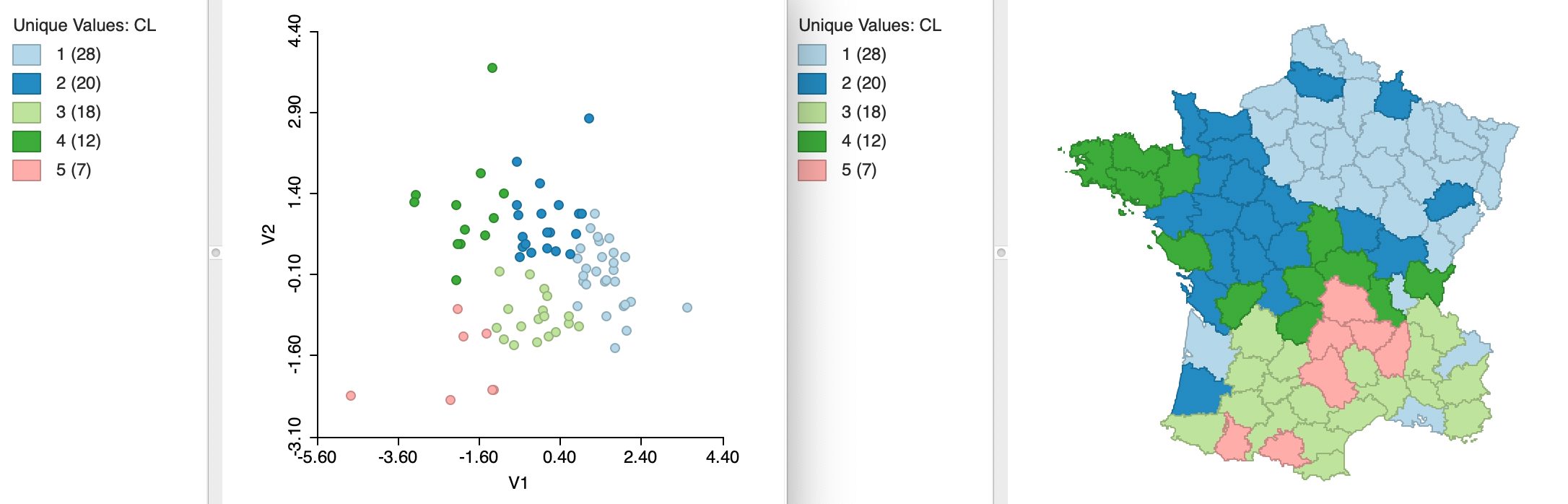
Figure 33: MDS plot and cluster map

Similarly, the summary results are the same, as shown in Figure 34, except that the signs of the cluster centers for V2 are the opposite of those for PC2 in Figure 32.

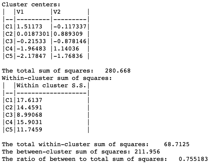
Figure 34: MDS cluster summary

Appendix

Equivalence of Euclidean distances and Sum of Squared Errors (SSE)

We start with the objective function as the within sum of squared distances. More precisely, this is expressed as one half the sum of the squared Euclidean distances for each cluster between all the pairs \(i-j\) that form part of the cluster \(h\), i.e., for all \(i \in h\) and \(j \in h\): \[W = (1/2) \sum_{h=1}^k \sum_{i \in h} \sum_{j \in h} ||x_i - x_j||^2.\] To keep things simple, we take the \(x\) as univariate, so we can ignore the more complex notation needed for higher order manipulations. This is without a loss of generality, since for multiple variables the Euclidean distance is simply the sum of the distances for each of the variables.

A fundamental identity exploited to move from the sum of all pairwised distances to the sum of squared deviations is that: \[(1/2) \sum_i \sum_j (x_i - x_j)^2 = n \sum_i (x_i - \bar{x})^2,\] where \(\bar{x}\) is the mean of \(x\). This takes a little algebra to confirm.

For each \(i\) in a given cluster \(h\), the sum over the \(j\) in the cluster is: \[\sum_{j \in h} (x_i - x_j)^2 = \sum_{j \in h} (x_i^2 - 2x_ix_j + x_j^2),\] or (dropping the \(\in h\) notation for simplicity), \[\sum_j x_i^2 - 2\sum_j x_i x_j + \sum_j x_j^2.\]

With \(n_h\) observations in cluster \(h\), \(\sum_j x_i^2 = n_h x_i^2\) (since \(x_i\) does not contain the index \(j\) and thus is simply repeated \(n_h\) times). Also, \(\sum_j x_j = n_h \bar{x}_h\), where \(\bar{x}_h\) is the mean of \(x\) for cluster \(h\) (\(\bar{x}_h = \sum_j x_j / n_h = \sum_i x_i / n_h\)). As a result, \(- 2 x_i \sum_j x_j = - 2 n_h x_i \bar{x}_h\), which yields: \[\sum_{j} (x_i - x_j)^2 = n_h x_i^2 - 2 n_h x_i \bar{x}_h + \sum_j x_j^2.\] Next, we proceed in the same way to compute the sum over all the \(i \in h\): \[\sum_i \sum_{j} (x_i - x_j)^2 = n_h \sum_i x_i^2 - 2 n_h \bar{x}_h \sum_i x_i + \sum_i \sum_j x_j^2\] Using the same approach as before, and since \(\sum_j x_j^2 = \sum_i x_i^2\), this becomes: \[\sum_i \sum_{j} (x_i - x_j)^2 = n_h \sum_i x_i^2 - 2 n_h^2 \bar{x}_h^2 + n_h \sum_i x_i^2 = 2 n_h \sum_i x_i^2 - 2 n_h^2 \bar{x}_h^2,\] or, \[\sum_i \sum_{j} (x_i - x_j)^2 = 2n_h^2 (\sum_i x_i^2 / n_h - \bar{x}_h^2).\] From the definition of the variance, we know that the following equality holds: \[\sigma^2 = (1/n_h) \sum_i (x_i - \bar{x}_h)^2 = \sum_i x_i^2 / n_h - \bar{x}_h^2.\] Therefore: \[\sum_i \sum_{j} (x_i - x_j)^2 = 2n_h^2 [(1/n_h) \sum_i (x_i - \bar{x}_h)^2] = 2n_h [ \sum_i (x_i - \bar{x}_h)^2 ],\] which gives the contribution of cluster \(h\) to the objective function as: \[(1/2) \sum_i \sum_{j} (x_i - x_j)^2 = n_h [ \sum_i (x_i - \bar{x}_h)^2 ].\]

For all the clusters jointly, the objective becomes: \[\sum_{h=1}^k n_h \sum_{i \in h} (x_i - \bar{x}_h)^2.\]

In other words, minimizing the sum of (one half) of all squared distances is equivalent to minimizing the sum of squared deviations from the mean in each cluster, the within sum of squared errors.

K-means worked example

We now provide the details behind the k-means algorithm portrayed in Figures 1 and 2. The coordinates of the seven points are given in the X and Y columns of Figure 35. The column labeled as SSE shows the squared distance from each point to the center of the point cloud, computed as the average of the X and Y coordinates (X=5.714, Y=5.143).¹¹ The sum of the squared distances constitutes the total sum of squared errors, or TSS, which equals 62.286 in this example. This value does not change as we iterate, since it pertains to all the observations taken together and ignores the cluster allocations.

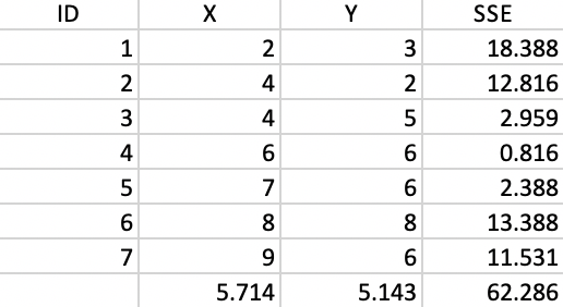
Figure 35: Worked example - basic data

The initialization consists of randomly picking two observations as starting points, one for each potential cluster. In this example, we take observations 4 and 7. Next, we compute the distance from each point to the two seeds and allocate each to the closest seed. The highlighted values in columns d_i4 and d_i7 in Figure 36 show how the first allocation consists of five observations in cluster 1 (1-5) and two observations in cluster 2 (6 and 7).

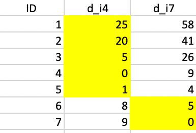
Figure 36: Squared distance to seeds

Next, we compute a central point for each cluster as the average of the respective X and Y coordinates. The SSE follows as the squared distance between each observation in the cluster and the central point, as listed in Figure 37. The sum of the total SSE in each cluster is the within sum of squares, WSS = 30.9 in this first step. Consequently, the between sum of squares BSS = TSS - WSS = 62.3 - 30.9 = 31.4. The associated ratio BSS/TSS, which is an indicator of the quality of the cluster is 0.50.

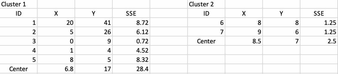
Figure 37: Step 1 - Summary characteristics

Next, we take the new cluster center points and again allocate each observation to the closest center. As shown in Figure 38, this results in observation 5 moving from cluster 1 to cluster 2, which now consists of three observations (cluster 1 has the remaining four).

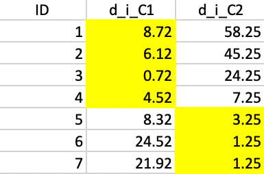
Figure 38: Squared distance to Step 1 centers

We compute the new cluster centers and calculate the associated SSE. As suggested by Figure 39, this results in a new WSS of 22.667, clearly an improvement of the objective function. The corresponding ratio of BSS/TSS becomes 0.64, also a clear improvement.

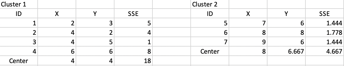
Figure 39: Step 2 - Summary characteristics

We repeat the process with the updated centers, which results in observation 4 moving from cluster 1 to cluster 2, as illustrated in Figure 40.

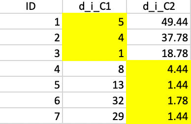
Figure 40: Squared distance to Step 2 centers

Figure 41 shows the new cluster centers and associated SSE. The updated WSS is 15.333, yielding a ratio BSS/TSS of 0.75.

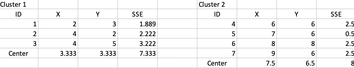
Figure 41: Step 3 - Summary characteristics

Finally, this latest allocation no longer results in a change, as shown Figure 42, so that we can conclude that we reached a local optimum.

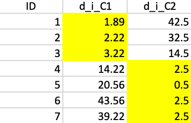
Figure 42: Squared distance to Step 3 centers

Figure 43 demonstrates that this is the same result as obtained by GeoDa with the default settings, but the Transformation set to Raw in order to use the actual coordinates.¹²

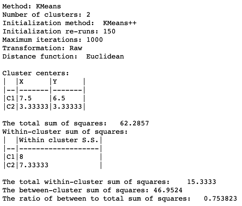
Figure 43: K-means results from GeoDa

References

Arthur, David, and Sergei Vassilvitskii. 2007. “k-means++: The Advantages of Careful Seeding.” In SODA 07, Proceedings of the Eighteenth Annual ACM-SIAM Symposium on Discrete Algorithms, edited by Harold Gabow, 1027–35. Philadelphia, PA: Society for Industrial and Applied Mathematics.

Dempster, A. P., N. M. Laird, and D. B. Rubin. 1977. “Maximum Likelihood from Incomplete Data via the EM Algorithm.” Journal of the Royal Statistical Society, Series B 39: 1–38.

Everitt, Brian S., Sabine Landau, Morven Leese, and Daniel Stahl. 2011. Cluster Analysis, 5th Edition. New York, NY: John Wiley.

Fränti, Pasi, and Sami Sieranoja. 2018. “K-Means Properties on Six Clustering Benchmark Datasets.” Applied Intelligence 48: 4743–59.

Han, Jiawei, Micheline Kamber, and Jian Pei. 2012. Data Mining (Third Edition). Amsterdam: MorganKaufman.

Hartigan, J. A., and M. A. Wong. 1979. “Algorithm AS 136: A k-means Clustering Algorithm.” Applied Statistics 28: 100–108.

Hartigan, John A. 1972. “Direct Clustering of a Data Matrix.” Journal of the American Statistical Association 67: 123–29.

———. 1975. Clustering Algorithms. New York, NY: John Wiley.

Hastie, Trevor, Robert Tibshirani, and Jerome Friedman. 2009. The Elements of Statistical Learning (2nd Edition). New York, NY: Springer.

Hoon, Michiel de, Seiya Imoto, and Satoru Miyano. 2017. “The C Clustering Library.” Tokyo, Japan: The University of Tokyo, Institute of Medical Science, Human Genome Center.

Jain, Anil K. 2010. “Data Clustering: 50 Years Beyond K-Means.” Pattern Recognition Letters 31 (8): 651–66.

Jain, Anil K., and Richard C. Dubes. 1988. Algorithms for Clustering Data. Englewood Cliffs, NJ: Prentice Hall.

James, Gareth, Daniela Witten, Trevor Hastie, and Robert Tibshirani. 2013. An Introduction to Statistical Learning, with Applications in R. New York, NY: Springer-Verlag.

Kaufman, L., and P. Rousseeuw. 2005. Finding Groups in Data: An Introduction to Cluster Analysis. New York, NY: John Wiley.

Lloyd, Stuart P. 1982. “Least Squares Quantization in PCM.” IEEE Transactions on Information Theory 28: 129–36.

Padilha, Victor A., and Ricardo J. G. B. Campello. 2017. “A Systematic Comparative Evaluation of Biclustering Techniques.” BMC Bioinformatics 18: 55. https://doi.org/10.1186/s12859-017-1487-1.

Tanay, Amos, Roded Sharan, and Ron Shamir. 2004. “Biclustering Algorithms: A Survey.” In Handbook of Computational Molecular Biology, edited by Srinivas Aluru, 26–21–17. Boca Raton, FL: Chapman & Hall/CRC.

Tibshirani, Robert, Guenther Walther, and Trevor Hastie. 2001. “Estimating the Number of Clusters in a Data Set via the Gap Statistic.” Journal of the Royal Statistical Society, Series B 63: 411–23.

---

1. University of Chicago, Center for Spatial Data Science – anselin@uchicago.edu↩︎

2. While we discuss dimension reduction and clustering separately, so-called biclustering techniques group both variables and observations simultaneously. While old, going back to an article by Hartigan (1972), these techniques have gained a lot of interest more recently in the field of gene expression analysis. For overviews, see, e.g., Tanay, Sharan, and Shamir (2004) and Padilha and Campello (2017).↩︎

3. The discussion in this section is loosely based on part of the presentation in Hastie, Tibshirani, and Friedman (2009) Chapter 14.↩︎

4. Since each pair is counted twice, the total sum is divided by 2. While this seems arbitrary at this point, it helps later on when we establish the equivalence between the Euclidean distances and the sum of squared errors.↩︎

5. As shown in Han, Kamber, and Pei (2012), p. 505, the k-means algorithm can be considered to be a special case of the so-called EM (expectation-maximization) algorithm of Dempster, Laird, and Rubin (1977). The expectation step consists of allocating each observation to its nearest cluster center, and the maximization step is the recalculation of those cluster centers for each new layout.↩︎

6. The drop-down list goes from 2 to 85, which may be insufficient in big data settings. Hence GeoDa now offers the option to enter a value directly.↩︎

7. The Z standardization subtracts the mean and divides by the standard deviation. Alternative standardizations are to use the mean absolute deviation, MAD, the range adjust or range standardization methods.↩︎

8. In the current implementation, the same summary method needs to be applied to all the variables.↩︎

9. The categories have been adjusted to keep the same color pattern as with the cluster map in Figure 19.↩︎

10. For a similar logic, see for example Chapter 2 in Everitt et al. (2011), where a visual inspection of two-dimensional scatter plots of principal components is illustrated as way to identify clusters.↩︎

11. Each squared distance is \((x_i - \bar{x})^2 + (y_i - \bar{y})^2\).↩︎

12. This is accomplished by loading a csv file with the coordinates as the data input in GeoDa.↩︎

GeoDa is maintained by lixun910. This page was generated by GitHub Pages using the Cayman theme by Jason Long.