Cluster Analysis (3)

Advanced Clustering Methods

Introduction

In this chapter, we consider some more advanced partitioning methods. First, we cover two variants of K-means, i.e., K-medians and K-medoids. These operate in the same manner as K-means, but differ in the way the central point of each cluster is defined and the manner in which the nearest points are assigned. In addition, we discuss spectral clustering, a graph partitioning method that can be interpreted as simultaneously implementing dimension reduction with cluster identification.

As implemented in GeoDa, these methods share almost all the same options with the partitioning and hierarchical clustering methods discussed in the previous chapters. These common aspects will not be considered again. We refer to the previous chapters for details on the common options and sensitivity analyses.

We continue to use the Guerry data set to illustrate k-medians and k-medoids, but introduce a new sample data set, spirals.csv, for the spectral clustering examples.

Objectives

• Understand the difference between k-median and k-medoid clustering

• Carry out and interpret the results of k-median clustering

• Gain insight into the logic behind the PAM, CLARA and CLARANS algorithms

• Carry out and interpret the results of k-medoid clustering

• Understand the graph-theoretic principles underlying spectral clustering

• Carry out and interpret the results of spectral clustering

GeoDa functions covered

• Clusters > K Medians
  • select variables
  • MAD standardization
• Clusters > K Medoids
• Clusters > Spectral

Getting started

The Guerry data set can be loaded in the same way as before.

The spirals data set is specifically designed to illustrate some of the special characteristics of spectral clustering. It is one of the GeoDaCenter sample data sets.

To activate this data set, you load the file spirals.csv and select x and y as the coordinates (the data set only has two variables), as in Figure 1. This will ensure that the resulting layer is represented as a point map.

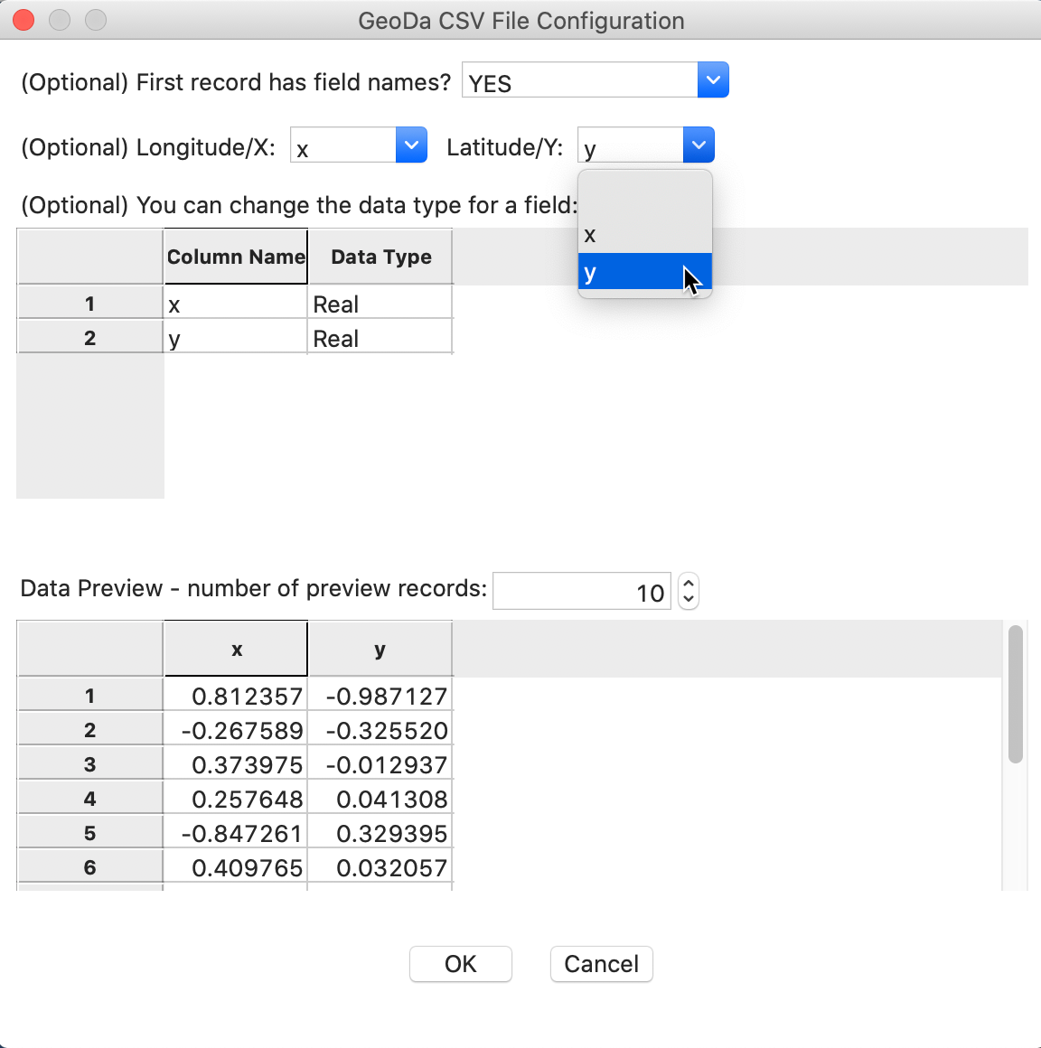
Figure 1: Spirals convert csv file to point map

The result shows the 300 points, consisting of two distinct but interwoven spirals, as in Figure 2.

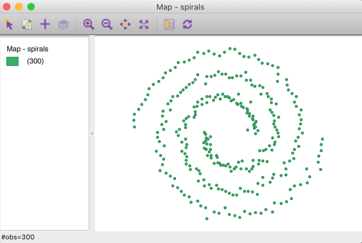
Figure 2: Spirals themeless point map

We will not be needing this data set until we cover spectral clustering. For k-medians and k-medoids, we use the Guerry data set.

K Medians

Principle

K-medians is a variant of k-means clustering. As a partitioning method, it starts by randomly picking k starting points and assigning observations to the nearest initial point. After the assignment, the center for each cluster is re-calculated and the assignment process repeats itself. In this way, k-medians proceeds in exactly the same manner as k-means. It is in fact also an EM algorithm.

In contrast to k-means, the central point is not the average (in multiattribute space), but instead the median of the cluster observations. The median center is computed separately for each dimension, so it is not necessarily an actual observation (similar to what is the case for the cluster average in k-means).

The objective function for k-medians is to find the allocation \(C(i)\) of observations \(i\) to clusters \(h = 1, \dots k\), such that the sum of the Manhattan distances between the members of each cluster and the cluster median is minimized: \[\mbox{argmin}_{C(i)} \sum_{h=1}^k \sum_{i \in h} || x_i - x_{h_{med}} ||_{L_1},\] where the distance metric follows the \(L_1\) norm, i.e., the Manhattan block distance.

K-medians is often confused with k-medoids. However, there is an important difference in that in k-medoids, the central point has to be one of the observations (Kaufman and Rousseeuw 2005). We consider k-medoids in the next section.

The Manhattan distance metric is used to assign observations to the nearest center. From a theoretical perspective, this is superior to using Euclidean distance since it is consistent with the notion of a median as the center (Hoon, Imoto, and Miyano 2017, 16).

In all other respects, the implementation and interpretation is the same as for k-means. To illustrate the logic, a simple worked example is provided in the Appendix.

GeoDa employs the k-medians implementation that is part of the C clustering library of Hoon, Imoto, and Miyano (2017).

Implementation

Just as the previous clustering techniques, k-medians is invoked from the Clusters toolbar. From the menu, it is selected as Clusters > K Medians, the second item in the classic clustering subset, as shown in Figure 3.

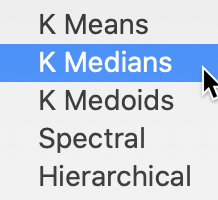
Figure 3: K Medians Option

This brings up the K Medians Clustering Settings dialog, with the Input options in the left-hand side panel, shown in Figure 4.

Variable Settings Panel

The user interface is identical to that for k-means, to which we refer for details. The main difference is that the Distance Function is Manhattan distance. In the example in Figure 4, we again select the same six variables as before, with the Number of Clusters set to 5 and all other options left to the default settings.

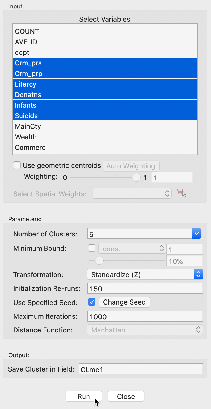
Figure 4: K Medians variable selection

Selecting Run brings up the cluster map and fills out the right-hand panel with some cluster characteristics, listed under Summary. The cluster categories are added to the Table using the variable name specified in the dialog (default is CL, in our example we use CLme1).

Cluster results

The cluster map is shown in Figure 5. The three largest clusters (they are labeled in sequence of their size) are well-balanced, with 24, 20 and 20 observations. The two others are much smaller, at 12 and 9. Interesting is that the clusters are also geographically quite compact, except for cluster 4, which consists of four different spatial subgroups. Cluster 2, in the south of the country, is actually fully contiguous (without imposing any spatial constraints). This is not the case for k-means.

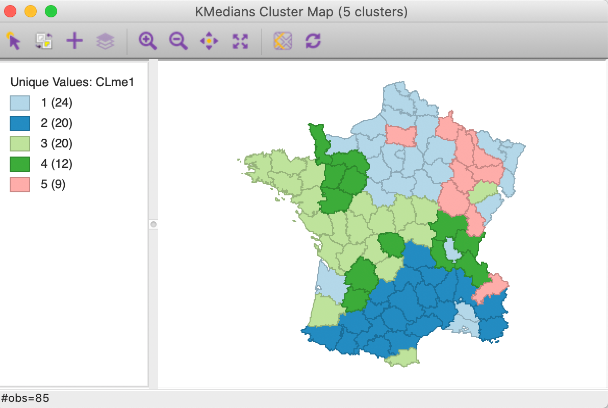
Figure 5: K Medians cluster map (k=5)

While the grouping may seem similar to what we obtained with other methods, this is in fact not the case. In Figure 6, the cluster map for k-means and k-medians are shown next to each other, with the labels for k-medians adjusted so as the get similar colors for each category. This highlights some of the important differences between the two methods. First of all, the size of the different “matching” clusters is not the same, nor is their geographic configuration. Considering the clusters for k-medians (with their new labels), we see that the largest cluster, with 24 observations, corresponds most closely with cluster 3 for k-means, which had 18 observations.

The closest match between the two results is for cluster 2, with only one mismatch out of 9 observations, although that cluster is much larger for k-means, with 19 observations. The worst match is for cluster 5, where only three observations are shared by the two methods for that cluster (out of 12). For the others, there is about a 3/4 match. In other words, the two methods pick out different patterns of similarity in the data. There is no “best” method, since each uses a different objective function. It is up to the analyst to decide which of the objectives makes most sense, in light of the goals of a particular study.

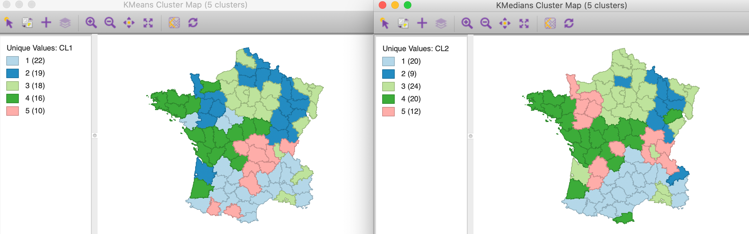
Figure 6: K Means and K Medians compared (k=5)

Further insight into the characteristics of the clusters obtained by the k-medians algorithm are found in the Summary panel on the right side of the settings dialog, shown in Figure 7.

The first set of items summarizes the settings for the analysis, such as the method used, the number of clusters and the various options for initialization, standardization, etc. Next follow the values for each of the variables associated with the median center of each cluster. These results are given in the original scale for the variables, whereas the other summary measures depend on the standardization used. Typically, the median center values are used to interpret the type of grouping that is obtained. This is not always easy, since one has to look for systematic combinations of variables with high or low values for the median so as to characterize the cluster.

The third set of items contains the summary statistics, using the squared difference and mean as the criterion, similar to what is used for k-means. Note that this is only for a general comparison, since this is not the criterion used in the objective function. So, in a sense, it gives a general impression of how the k-medians results compare using the standard used for k-means. In our example, we obtain a ratio of between to total sum of squares of 0.447, compared to 0.497 for k-means (with the default settings). This does not mean that the k-medians result is worse than that for k-means, but it gives a sense of how it performs under a different criterion that what it is optimized for.

The final set of summary characteristics are the proper ones for the objective of minimizing the within-cluster Manhattan distance relative to the cluster median. The total sum of the distances is 372.318. This is the sum of the distances between all observations and the overall median (using the z-standardized values for the variables). For k-medians, the objective is to decrease this value by grouping the observations into clusters with their own medians. The within-cluster total distance is listed for each cluster. In our results, there is quite a range in these values, going from 15.97 in the smallest cluster (with only 9 observations) to 70.49 in cluster 3 (with 20 observations). Clusters 1 and 2, that are larger or equal to the size of cluster 3, have a much better fit. This is also reflected in the average within-cluster distance results, with the smallest value of 1.77 for C5, followed by 2.61 for C1. Interestingly, the latter has about double the total distance compared to C4, but its average is better (2.61 compared to 2.84). The averages correct for the size of the cluster and are thus a good comparative measure of fit.

The total of the within-cluster distances is 250.399, a decrease of 121.9 from the original total. As a fraction of the original total, the final result is 0.673. When comparing results for different values of k, we would look for a bend in the elbow plot as this ratio decreases with increasing values of k.

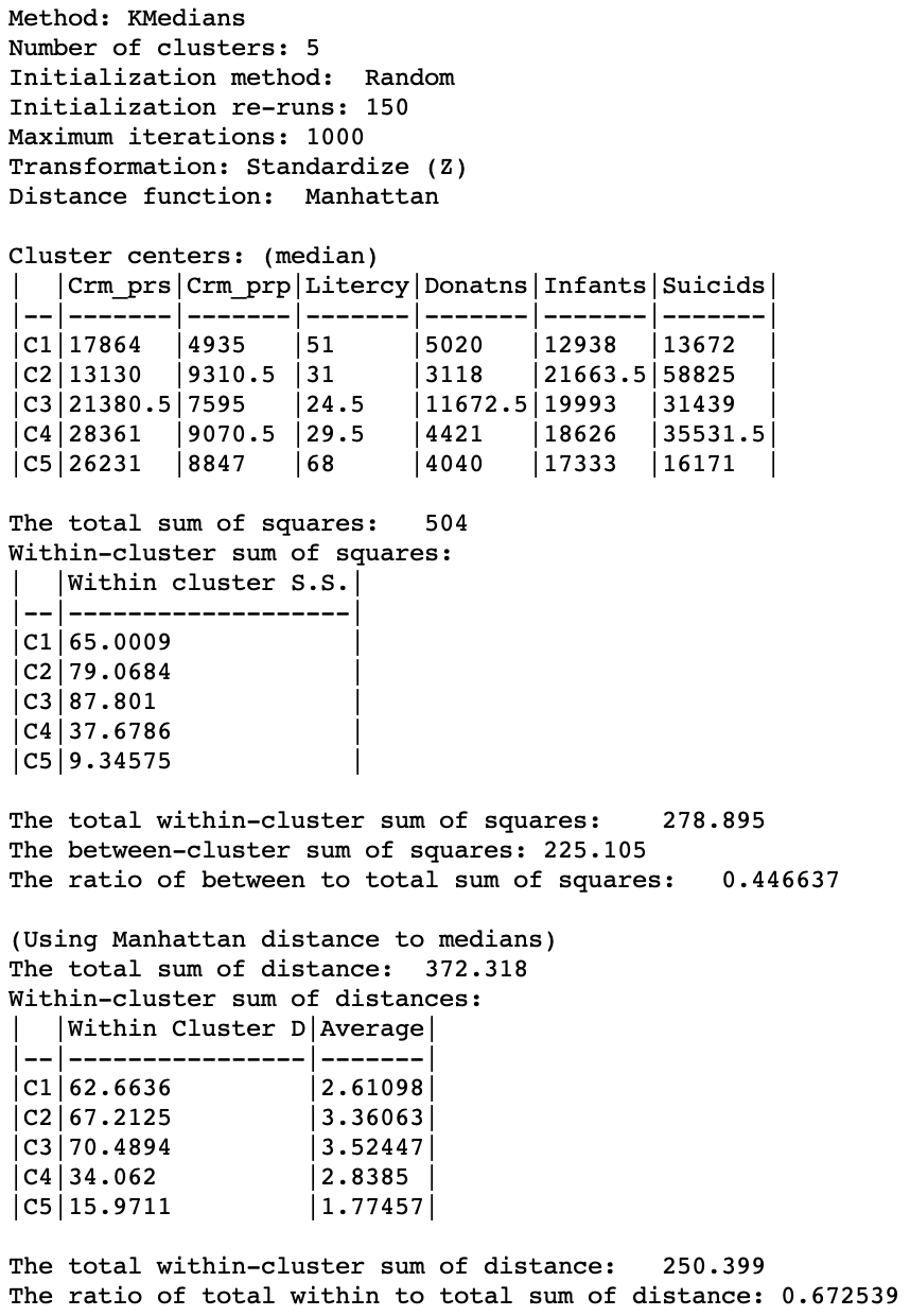
Figure 7: K Medians cluster characteristics (k=5)

Options and sensitivity analysis

The variables settings panel contains all the same options as for k-means, except that initialization is always by randomization, since there is no k-means++ method for k-medians. One option that is particularly useful in the context of k-medians (and k-medoids) is the use of a different standardization.

MAD standardization

The default z-standardization uses the mean and the variance of the original variables. Both of these are sensitive to the influence of outliers. Since the use of Manhattan distance and the median center for clusters in k-medians already reduces the effect of such outliers, it makes sense to also use a standardization that is less sensitive to those. We considered range standardization in the discussion of k-means. Here, we look at the mean absolute deviation, or MAD. As usual, this is selected as one of the Transformation options, as shown in Figure 8.

Figure 8: MAD variable standardization

The resulting cluster map and summary characteristics are shown in Figures 9 and 10.

The main effect seems to be on the largest cluster, which grows from 24 to 27 observations, mostly at the expense of what was the second largest cluster (which goes from 20 to 18 observations). As a result, none of the clusters are fully contiguous any more.

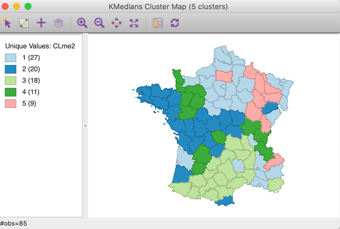
Figure 9: K Medians cluster map - MAD standardization (k=5)

The distance measures listed in the summary show a different starting point, with a total distance sum of 490.478, compared to 372.318 for z-standardization (recall that these measures are expressed in whatever units were used for the standardization). Therefore, the values for the within-cluster distance and their averages are not directly comparable to those using z-standardization. Only relative comparisons are warranted.

In the end, the total within-clusters are reduced to 0.677 of the original total, a slightly worse result than for z-standardization. However, this does not necessarily mean that z-standardization is superior. The choice of a particular transformation should be made within the context of the substantive research question. When no strong guidelines exist, a sensitivity analysis comparing, for example, z-standardization, range standardization and MAD may be the best strategy.

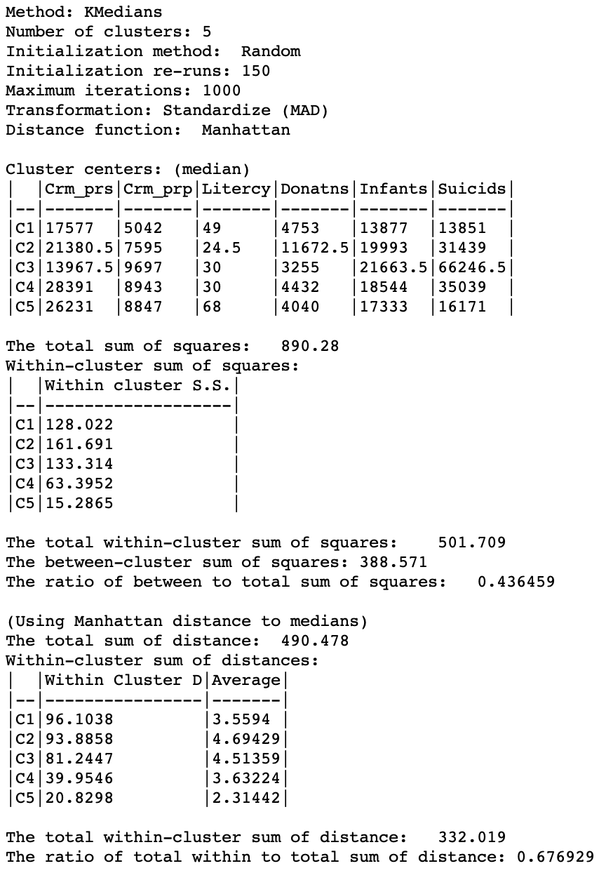
Figure 10: K Medians cluster characteristics - MAD standardization (k=5)

K Medoids

Principle

The objective of the k-medoids algorithm is to minimize the sum of the distances from the observations in each cluster to a representative center for that cluster. In contrast to k-means and k-medians, those centers do not need to be computed, since they are actual observations. As a consequence, k-medoids works with any dissimilarity matrix. If actual observations are available (as in the implementation in GeoDa), the Manhattan distance is the preferred metric, since it is less affected by outliers. In addition, since the objective function is based on the sum of distances instead of their squares, the influence of outliers is even smaller.²

The objective function can thus be expressed as finding the cluster assignments \(C(i)\) such that: \[\mbox{argmin}_{C(i)} \sum_{h=1}^k \sum_{i \in h} d_{i,h_c},\] where \(h_c\) is a representative center for cluster \(h\) and \(d\) is the distance metric used (from a dissimilarity matrix). As was the case for k-means (and k-medians), the problem is NP hard and an exact solution does not exist.³

The main approach to the k-medoids problem is the so-called partitioning around medoids (PAM) algorithm of Kaufman and Rousseeuw (2005). The logic underlying the PAM algorithm consists of two stages, BUILD and SWAP. In the first, a set of \(k\) starting centers are selected from the \(n\) observations. In some implementations, this is a random selection, but Kaufman and Rousseeuw (2005), and, more recently Schubert and Rousseeuw (2019) prefer a step-wise procedure that optimizes the initial set. The main part of the algorithm proceeds in a greedy iterative manner by swapping a current center with a candidate from the remaining non-centers, as long as the objective function can be improved. Detailed descriptions are given in Kaufman and Rousseeuw (2005), Chapters 2 and 3, as well as in Hastie, Tibshirani, and Friedman (2009), pp. 515-520, and Han, Kamber, and Pei (2012), pp. 454-457. A brief outline is presented next.

The PAM algorithm for k-medoids

The BUILD phase of the algorithm consists of identifying \(k\) observations out of the \(n\) and assigning them to be cluster centers \(h\), with \(h = 1, \dots, k\). This can be accomplished by randomly selecting the starting points a number of times and picking the one with the best (lowest) value for the objective function, i.e., the lowest sum of distances from observations to their cluster centers.

As a preferred option, Kaufman and Rousseeuw (2005) outline a step-wise approach that starts by picking the center, say \(h_1\), that minimizes the overall sum. This is readily accomplished by taking the observation that corresponds with the smallest row or column sum of the dissimilarity matrix. Next, each additional center (for \(h = 2, \dots, k\)) is selected that maximizes the difference between the closest distance to existing centers and the new potential center for all points (in practice, for the points that are closer to the new center than to existing centers).

For example, given the distance to \(h_1\), we compute for each of the remaining \(n - 1\) points \(j\), its distance to all candidate centers \(i\) (i.e., the same \(n-1\) points). Consider a \((n-1) \times (n-1)\) matrix where each observation is both row (\(i\)) and column (\(j\)). For each column \(j\), we compare the distance to the row-element \(i\) with the distance to the nearest current center for \(j\). In the second iteration, this is simply the distance to \(h_1\), but at later iterations different \(j\) will have different centers closest to them. If \(i\) is closer to \(j\) than its current closest center, then \(d_{j,h_1} - d_{ji} > 0\). The maximum of this difference and 0 is entered in position \(i,j\) of the matrix (in other words, negatives are not counted). The row \(i\) with the largest row sum (i.e., the largest improvement in the objective function) is selected as the next center.

At this point, the distance for each \(j\) to its nearest center is updated and the process starts anew for \(n-2\) observations. This continues until \(k\) centers have been picked.

In the SWAP phase, we consider all possible pairs that consist of a cluster center \(i\) and one of the \(n - k\) non-centers, \(r\), for a possible swap, for a total of \(k \times (n-k)\) pairs \((i, r)\).

We proceed by evaluating the change to the objective function that would follow from removing center \(i\) and replacing it with \(r\), as it affects the allocation of each other point (non-center and non-candidate) to either the new center \(r\) or one of the current centers \(g\) (but not \(i\), since that is no longer a center). This contribution follows from the change in distance that may occur between \(j\) and its new center. Those values are summed over all \(n - k - 1\) points \(j\). We compute this sum for each pair \(i, r\) and find the minimum over all pairs. If this minimum is negative (i.e., it decreases the total sum of distances), then \(i\) and \(r\) are swapped. This continues until there are no more improvements, i.e., the minimum is positive.

We label the change in the objective from \(j\) from a swap between \(i\) and \(r\) as \(C_{jir}\). The total improvement for a given pair \(i, r\) is the sum over all \(j\), \(T_{ir} = \sum_j C_{jir}\). The pair \(i, r\) is selected for a swap for which the minimum over all pairs of \(T_{ir}\) is negative, i.e., \(\mbox{argmin}_{i,r} T_{ir} < 0\).

The computational burden associated with this algorithm is quite high, since at each iteration \(k \times (n - k)\) pairs need to be evaluated. On the other hand, no calculations other than comparison and addition/subtraction are involved, and all the information is in the (constant) dissimilarity matrix.

To compute the net change in the objective function due to \(j\) that follows from a swap between \(i\) and \(r\), we distinguish between two cases. In one, \(j\) belongs to the cluster \(i\), such that \(d_{ji} < d_{jg}\) for all other centers \(g\). In the other case, \(j\) belongs to a different cluster, say \(g\), and \(d_{jg} < d_{ji}\). In both instances, we have to compare the distances from the nearest current center (\(i\) or \(g\)) to the distance to the candidate point, \(r\). Note that we don’t actually have to carry out the cluster assignments, since we compare the distance for all \(n - k - 1\) points \(j\) to the closest center (\(i\) or \(g\)) and the candidate center \(r\). All this information is contained in the elements of the dissimilarity matrix.

Consider the first case, where \(j\) is not part of the cluster \(i\), as in Figure 11. We see two scenarios for the configuration of the point \(j\), labeled \(j1\) and \(j2\). These points are closer to \(g\) than to \(i\), since they are not part of the cluster around \(i\). We now need to check whether \(j\) is closer to \(r\) than to its current cluster center \(g\). If \(d_{jg} \leq d_{jr}\), then nothing changes and \(C_{jir} = 0\). This is the case for point \(j1\). The dashed red line gives the distance to the current center \(g\) and the dashed green line gives the distance to \(r\). Otherwise, if \(d_{jr} < d_{jg}\), as is the case for point \(j2\), then \(j\) is assigned to \(r\) and \(C_{jir} = d_{jr} - d_{jg}\), a negative value, which decreases the overall cost. In the figure, we can compare the length of the dashed red line to the length of the solid green line, which designates a re-assignment to the candidate center \(r\).

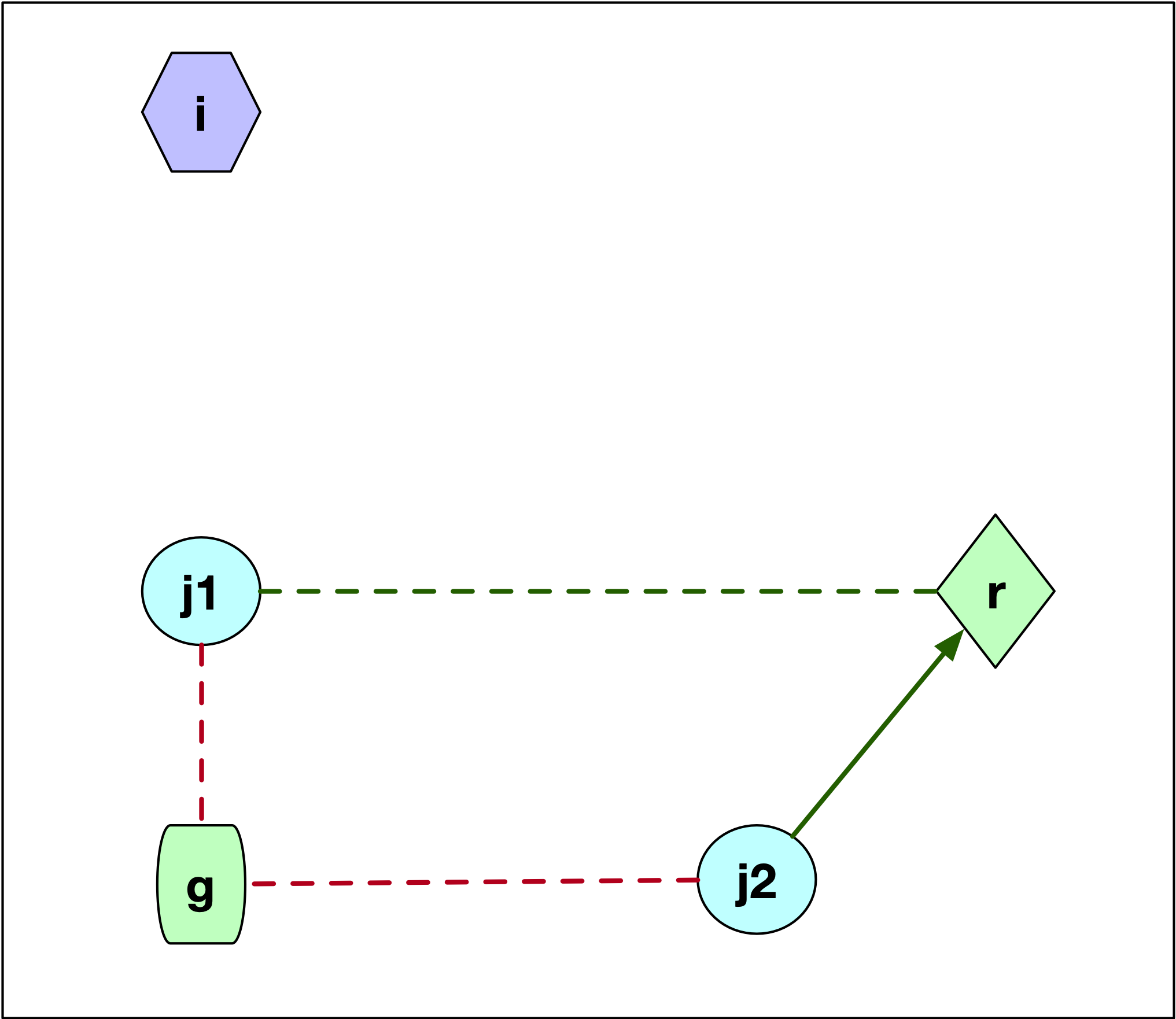
Figure 11: PAM SWAP - case 1

When \(j\) is part of cluster \(i\), then we need to assess whether \(j\) would be assigned to \(r\) or to the next closest center, say \(g\), since \(i\) would no longer be part of the cluster centers. This is illustrated in Figure 12, which has three options for the location of \(j\) relative to \(g\) and \(r\). In the first case, illustrated by point \(j1\), \(j\) is closer to \(g\) than to \(r\). This is illustrated by the difference in length between the dashed green line (\(d_{j1r}\)) and the solid green line (\(d_{j1g}\)). More precisely, \(d_{jr} \geq d_{jg}\) so that \(j\) is now assigned to \(g\). The change in the objective is \(C_{jir} = d_{jg} - d_{ji}\). This value is positive, since \(j\) was part of cluster \(i\) and thus was closer to \(i\) than to \(g\) (compare the length of the red dashed line between \(j1\) and \(i\) and the length of the line connecting \(j1\) to \(g\)).

If \(j\) is closer to \(r\), i.e., \(d_{jr} < d_{jg}\), then we can distinguish between two cases, one depicted by \(j2\), the other by \(j3\). In both instances, the result is that \(j\) is assigned to \(r\), but the effect on the objective differs. In the Figure, for both \(j2\) and \(j3\) the dashed green line to \(g\) is longer than the solid green line to \(r\). The change in the objective is the difference between the new distance and the old one (\(d_{ji}\)), or \(C_{jir} = d_{jr} - d_{ji}\). This value could be either positive or negative, since what matters is that \(j\) is closer to \(r\) than to \(g\), irrespective of how close \(j\) might have been to \(i\). For point \(j2\), the distance to \(i\) (dashed red line) was smaller than the new distance to \(r\) (solid green line), so \(d_{jr} - d_{ji} > 0\). In the case of \(j3\), the opposite holds, and the length to \(i\) (dashed red line) is larger than the distance to the new center (solid green line). In this case, the change to the objective is \(d_{jr} - d_{ji} < 0\).

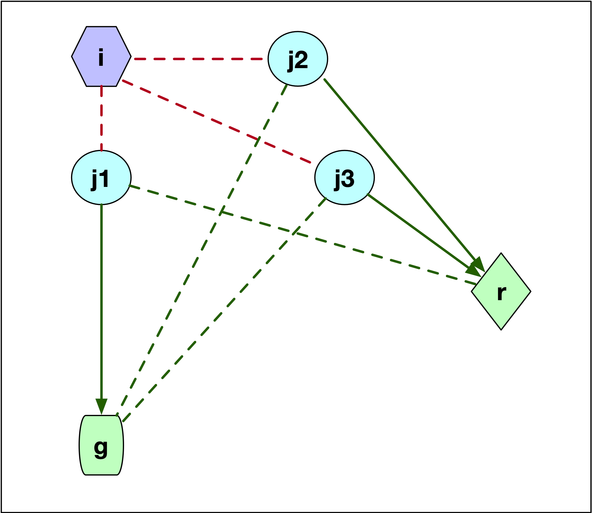
Figure 12: PAM SWAP - case 2

After the value for \(C_{jir}\) is computed for all \(j\), the sum \(T_{ir}\) is evaluated. This is repeated for every possible pair \(i,r\) (i.e., \(k\) centers to be replaced by \(n-k\) candidate centers). If the minimum over all pairs is negative, then \(i\) and \(r\) for the selected pair are exchanged, and the process is repeated. If the minimum is positive, the iterations end.

An illustrative worked example is given in the Appendix.

Improving on the PAM algorithm

The complexity of each iteration in the original PAM algorithm is of the order \(k \times (n - k)^2\), which means it will not scale well to large data sets with potentially large values of \(k\). To address this issue, Kaufman and Rousseeuw (2005) proposed the algorithm CLARA, based on a sampling strategy.

Instead of considering the full data set, a subsample is drawn. Then PAM is applied to find the best \(k\) medoids in the sample. Next, the distance from all observations (not just those in the sample) to their closest medoid is computed to assess the overall quality of the clustering.

The sampling process can be repeated for several more samples (keeping the best solution from the previous iteration as part of the sampled observations), and at the end the best solution is selected. While easy to implement, this approach does not guarantee that the best local optimum solution is found. In fact, if one of the best medoids is never sampled, it is impossible for it to become part of the final solution. Note that as the sample size is increased, the results will tend to be closer to those given by PAM.⁴

In practical applications, Kaufman and Rousseeuw (2005) suggest to use a sample size of 40 + 2k and to repeat the process 5 times.⁵

In Ng and Han (2002), a different sampling strategy is outlined that keeps the full set of observations under consideration. The problem is formulated as finding the best node in a graph that consists of all possible combinations of \(k\) observations that could serve as the \(k\) medoids. The nodes are connected by edges to the \(k \times (n - k)\) nodes that differ in one medoid (i.e., for each edge, one of the \(k\) medoid nodes is swapped with one of the \(n - k\) candidates).

The algorithm CLARANS starts an iteration by randomly picking a node (i.e., a set of \(k\) candidate medoids). Then, it randomly picks a neighbor of this node in the graph. This is a set of \(k\) medoids where one is swapped with the current set. If this leads to an improvement in the cost, then the new node becomes the new start of the next set of searches (still part of the same iteration). If not, another neighbor is picked and evaluated, up to maxneighbor times. This ends an iteration.

At the end of the iteration the cost of the last solution is compared to the stored current best. If the new solution constitutes an improvement, it becomes the new best. This search process is carried out a total of numlocal iterations and at the end the best overall solution is kept. Because of the special nature of the graph, not that many steps are required to achieve a local minimum (technically, there are many paths that lead to the local minimum, even when starting at a random node).

To make this concept more concrete, consider the toy example used in the Appendix, which has 7 observations. To construct k=2 clusters, any pair of 2 observations from the 7 could be considered a potential medoid. All those pairs constitute the nodes in the graph. The total number of nodes is given by the binomial coefficient \({n}\choose{k}\). In our example, \({{7}\choose{2}} = 21\).

Each of the 21 nodes in the graph has \(k \times (n - k) = 2 \times 5 = 10\) neighbors that differ only in one medoid connected with an edge. In our example, let’s say we pick (4,7) as a starting node, as we did in the worked example. It will be connected to all the nodes that differ by one medoid, i.e., either 4 or 7 is replaced (swapped in PAM terminology) by one of the \(n - k = 5\) remaining nodes. Specifically, this includes the following 10 neighbors: 1-7, 2-7, 3-7, 5-7, 6-7, and 4-1, 4-2, 4-3, 4-5 and 4-6. Rather than evaluating all 10 potential swaps, as we did for PAM, only a maximum number (maxneighbor) are evaluated. At the end of those evaluations, the best solution is kept. Then the process is repeated, up to the specified total number of iterations, which Ng and Han (2002) call numlocal.

Let’s say we set maxneighbors to 2. Consider the first step of the random evaluation in which we randomly pick the pair 4-5 from the neighboring nodes. In other words, we replace 7 in the original set by 5. Using the values from the worked example in the Appendix, we have \(T_{45} = 3\), a positive value, so this does not improve the objective function. We increase the iteration count (for maxneighbors) and pick a second random node, say 4-2 (i.e., now replacing 7 by 2). Now the value \(T_{42} = -3\) so the objective is improved to 20-3 = 17. Since we have reached the end of maxneighbors, we store this value as best and now repeat the process, picking a different random starting point. We continue this until we have obtained numlocal local optima and keep the best overall solution.

Based on their numerical experiments, Ng and Han (2002) suggest that no more than 2 iterations need to be pursued (i.e., numlocal = 2), with some evidence that more operations are not cost-effective. They also suggest a sample size of 1.25% of \(k \times (n-k)\).⁶

Both CLARA and CLARANS are large data methods, since for smaller data sizes (say < 100), PAM will be feasible and obtain better solutions (since it implements an exhaustive evaluation).

Further speedup of PAM, CLARA and CLARANS is outlined in Schubert and Rousseeuw (2019), where some redundancies in the comparison of distances in the SWAP phase are removed. In essence, this exploits the fact that observations allocated to a medoid that will be swapped out, will move to either the second closest medoid or to the swap point. Observations that are not currently allocated to the medoid under consideration will either stay in their current cluster, or move to the swap point, depending on how the distance to their cluster center compares to the distance to the swap point. These ideas shorten the number of loops that need to be evaluated and allow the algorithms to scale to much larger problems (details are in Schubert and Rousseeuw 2019, 175). In addition, they provide and option to carry out the swaps for all current k medoids simultaneously, similar to the logic in k-means (this is implemented in the FASTPAM2 algorithm, see Schubert and Rousseeuw 2019, 178).

A second improvement in the algorithm pertains to the BUILD phase. The original approach is replaced by a so-called Linear Approximative BUILD (LAB), which achieves linear runtime in \(n\). Instead of considering all candidate points, only a subsample from the data is used, repeated \(k\) times (once for each medoid).

The FastPAM2 algorithm tends to yield the best cluster results relative to the other methods, in terms of the smallest sum of distances to the respective medoids. However, especially for large n and large k, FastCLARANS yields much smaller compute times, although the quality of the clusters is not as good as for FastPAM2. FastCLARA is always much slower than the other two. In terms of the initialization methods, LAB tends to be much faster than BUILD, especially for larger n and k.

The FastPAM2, FastCLARA and FastCLARANS algorithms from Schubert and Rousseeuw (2019) were ported to C++ in GeoDa from the original Java code by the authors.⁷

Implementation

K-medoids is invoked from the Clusters toolbar, as the third item in the classic clustering subset, as shown in Figure 13. Alternatively, from the menu, it is selected as Clusters > K Medoids.

Figure 13: K Medoids Option

This brings up the usual variable settings panel.

Variable Settings Panel

The variable settings panel in Figure 14 has the by now familiar layout for the input section. It is identical to that for k-medians, except for the Method selection and the associated options. In our example with the same six variables as before (z-standardized), we use the default method of FastPAM. The default Initialization Method is LAB, with BUILD available as an alternative. In practice, LAB is much faster than BUILD.

There are no other options to be set, since the PAM algorithm proceeds with an exhaustive search in the SWAP phase, after an initial set of medoids is selected.

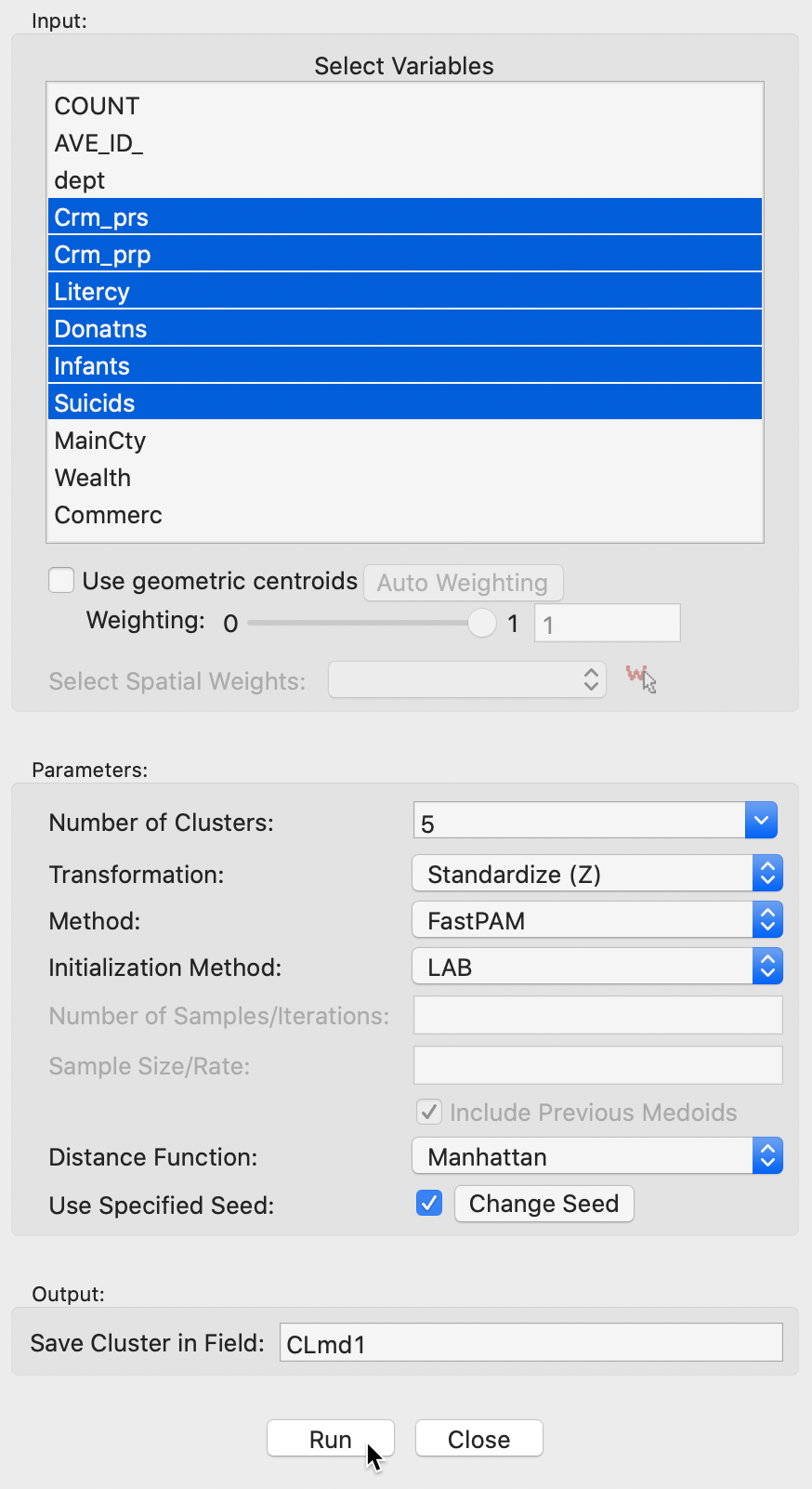
Figure 14: K Medoids variable selection

Clicking on Run brings up the cluster map, as well as the usual cluster characteristics in the right-hand panel. In addition, the cluster classifications are saved to the table using the variable name specified in the dialog (here CLmd1).

Cluster results

The cluster map in Figure 15 show results that are fairly similar to k-medians, although different in some important respects. In essence, the first cluster changes slightly, now with 26 members, while CL2 and CL3 swap places. The new CL2 has 21 members (compared to 20 for CL2 in k-median) and CL3 has 18 (compared to 20 for CL2 in k-median).

The two smallest clusters have basically the same size in both applications, but their match differs considerably. CL4 has no overlap between the two methods. On the other hand, CL5 is mostly the same between the two (7 out of 9 members in common). As we have pointed out before, this highlights how the various methods pick up different aspects of multi-attribute similarity. In many applications, k-medoids is preferred over k-means, since it tends to be less sensitive to outliers.

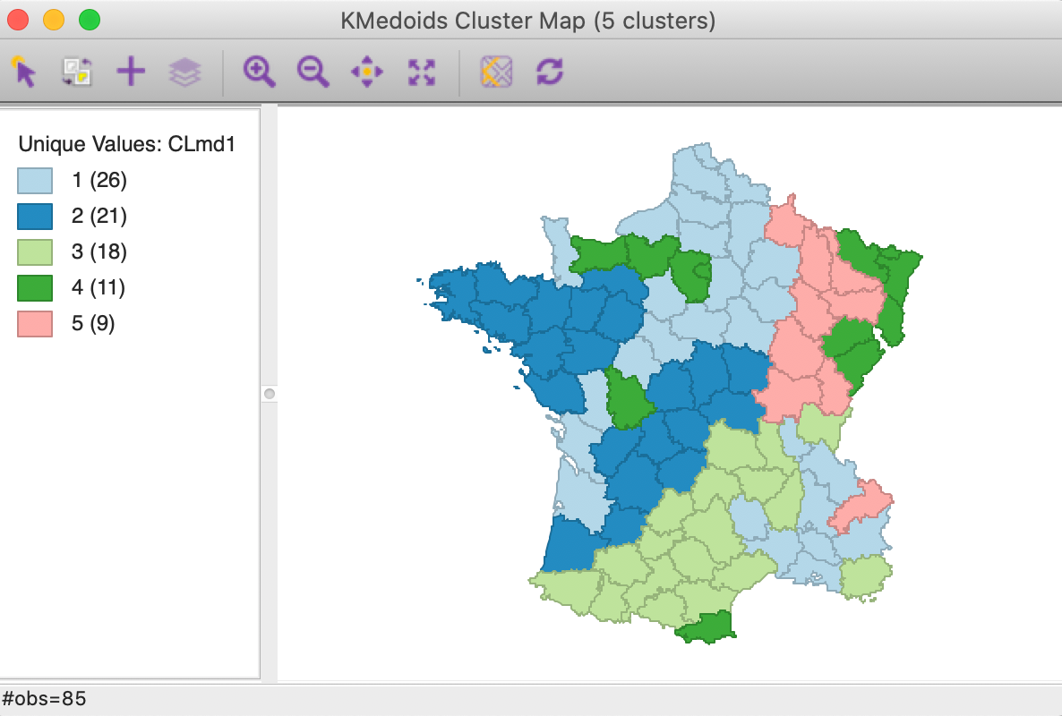
Figure 15: K Medoids cluster map (k=5)

One additional useful characteristic of the k-medoids approach is that the cluster centers are actual observations. In Figure 16, these are highlighted for our example. Note that these observations are centers in multi-attribute space, and clearly not in geographical space (we address this in the next chapter).

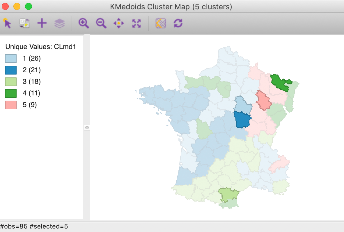
Figure 16: K Medoids cluster centers (k=5)

A more meaningful substantive interpretation of the cluster centers can be obtained from the cluster characteristics in Figure 17. Below the usual listing of methods and options, the observation numbers of the cluster medoids are given. These can be used to select the corresponding observations in the table.⁸ As before, the values for the different variables in each cluster center are listed, but now these correspond to actual observations, so we can also look these up in the data table.

While these values are expressed in the original units, the remainder of the summary characteristics are in the units used for the specified standardization, z-standardized in our example. First are the results for the within and between sum of squares. The summary ratio is 0.414, slightly worse than for k-median (but recall that this is not the proper objective function).

The point of departure for the within-cluster distances is the total distance to the overall medoid for the data. This is the observation for which the sum of distances from all other observations is the smallest (i.e., the observation with the smallest row or column sum of the elements in the distance matrix).

In our example, the within-cluster distances to each medoid and their averages show fairly tight clusters for CL1 and CL5, and less so for the other three. The original total distance decreases from 398.5 to 265.1, a ratio of 0.665, compared to 0.673 for k-median. This would suggest a slightly greater success at reducing the overall sum of distances (smaller values are better).

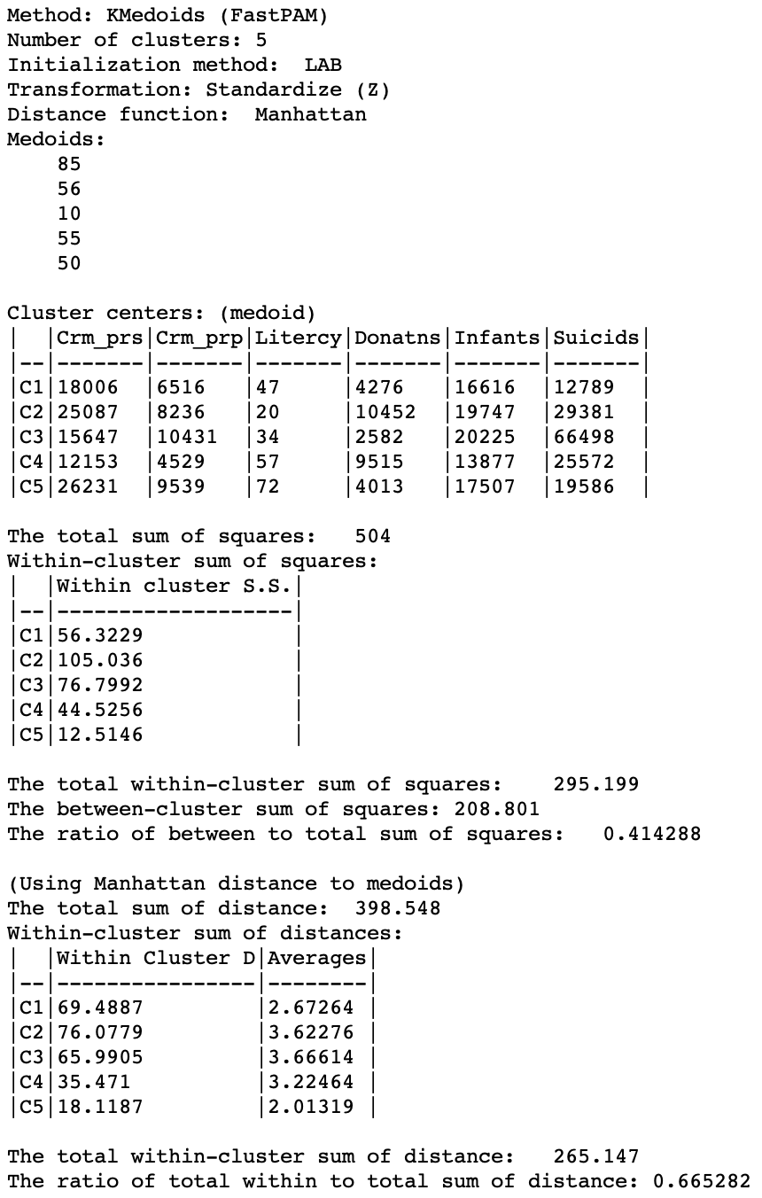
Figure 17: K Medoids cluster characteristics (k=5)

Options and sensitivity analysis

The main option for k-medoids is the choice of the Method. As shown in Figure 18, in addition to the default FastPAM, the algorithms FastCLARA and FastCLARANS are available as well. The latter two are large data methods and they will always perform (much) worse than FastPAM in small to medium-sized data sets. In our example, it would not be appropriate to use these methods, but we provide a brief illustration anyway to highlight the deterioration in the solutions found.

In addition, there is a choice of Initialization Method between LAB and BUILD. In most circumstances, LAB is the preferred option, but BUILD is included for the sake of completeness and to allow for a full range of comparisons.

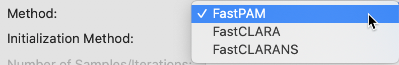
Figure 18: K Medoids method options

CLARA

The two main parameters that need to be specified for the CLARA method are the number of samples considered (by default set to 2) and the sample size. Since n < 100 in our example, the latter is set to 40+2K = 50, shown in Figure 19. In addition, the option to include the best previous medoids in the sample is checked.

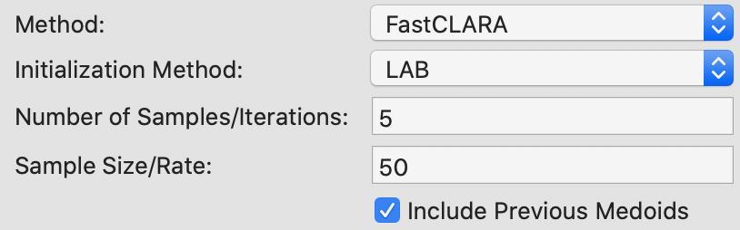
Figure 19: K Medoids CLARA parameters

The resulting cluster map is given in Figure 20, with associated cluster characteristics in Figure 21.

The main effect seems to be on CL4, which, even though it has the same number of members as for PAM, they are in totally different locations. CL1 increases its membership from 26 to 30. CL2 and CL3 shrink somewhat, mostly due to the (new) presence of the members of CL4. CL5 does not change.

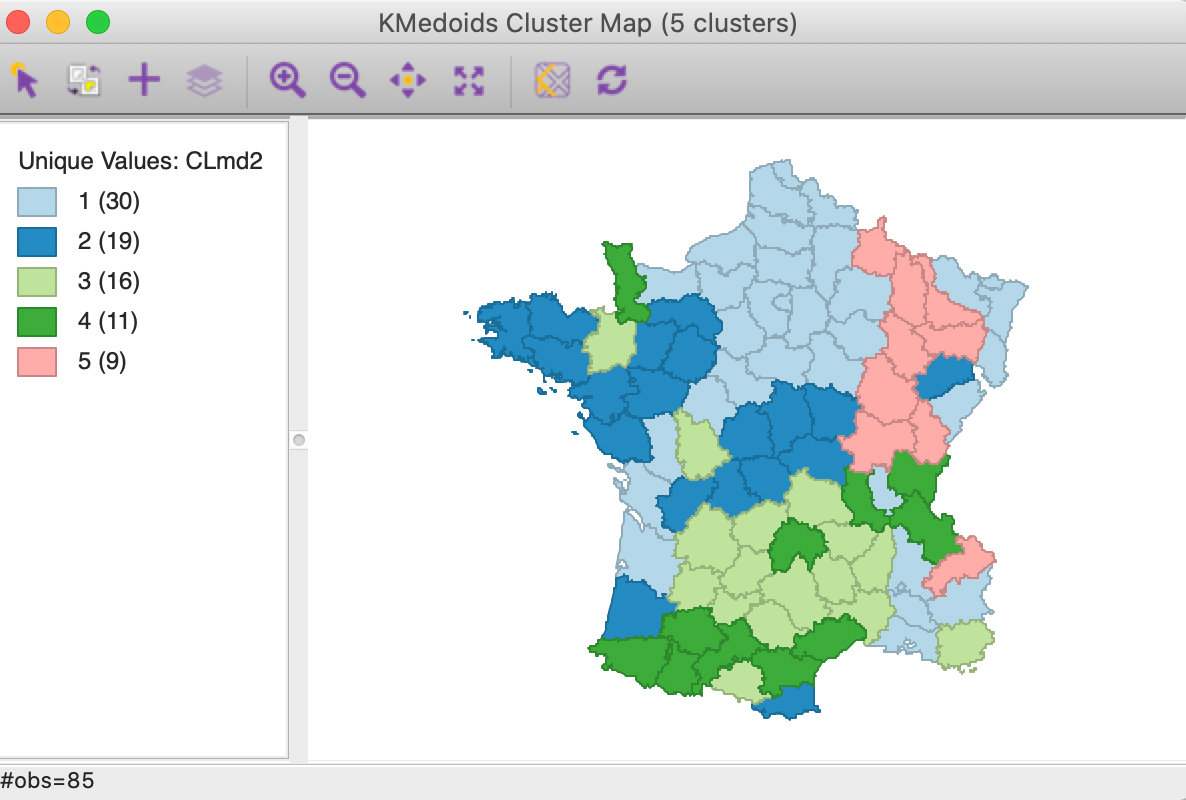
Figure 20: K Medoids CLARA cluster map (k=5)

As the summary characteristics show, CL3 and CL4 now have different medoids. Overall, there is a slight deterioration of the quality of the clusters, with the total within-cluster distance now 268.9 (compared to 265.1), for a ratio of 0.675 (compared to 0.665).

In this example, the use of a sample instead of the full data set does not lead to a meaningful deterioration of the results. This is not totally surprising, since the sample size of 50 is almost 59% of the total sample size. For larger data sets with k=5, the sample size will remain at 50, thus constituting a smaller and smaller share of the actual observations as the sample size increases.⁹

To illustrate the effect of sample size, we can set its value to 30. This results in a much larger overall within sum of distances of 273.9, with a ratio of 0.687 (details not shown). On the other hand, if we set the sample size to 85, then we obtain the exact same results as for PAM.

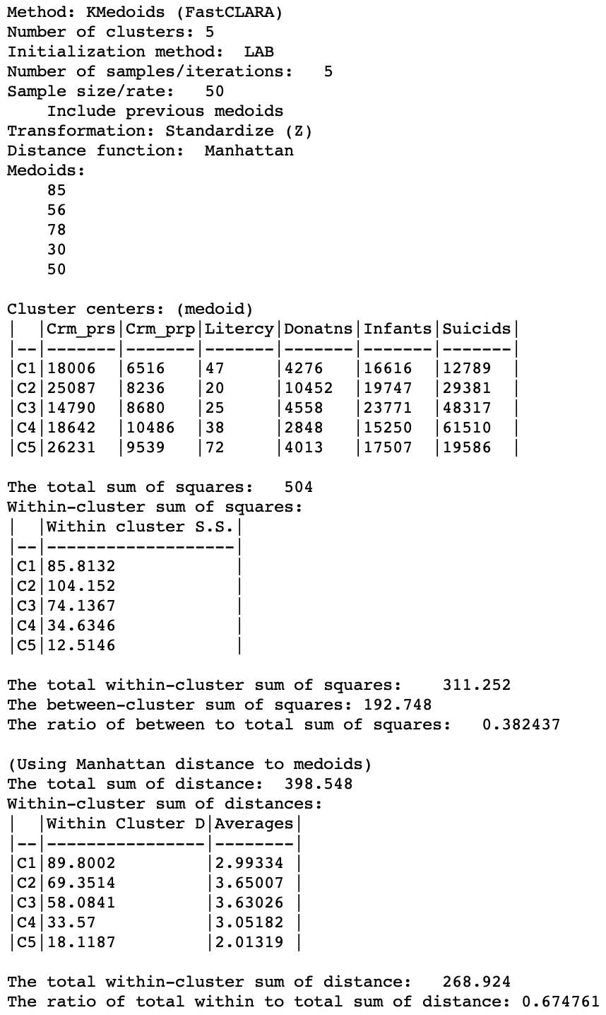
Figure 21: K Medoids CLARA cluster characteristics (k=5)

CLARANS

For CLARANS, the two relevant parameters pertain to the number of iterations and the sample rate, as shown in Figure 22. The former corresponds to the numlocal parameter in Ng and Han (2002), i.e., the number of times a local optimum is computed (default = 2). The sample rate pertains to the maximum number of neighbors that will be randomly sampled in each iteration (maxneighbors in the paper). This is expressed as a fraction of \(k \times (n - k)\). We use the value of 0.025 recommended by Schubert and Rousseeuw (2019), which yields a maximum neighbors of 10 (0.025 x 400) for each iteration in our example. Unlike PAM and CLARA, there is no initialization option.

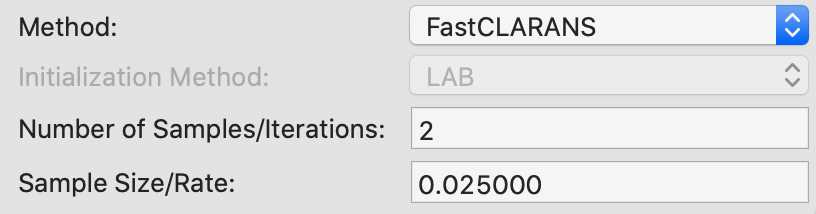
Figure 22: K Medoids CLARANS parameters

The results are presented in Figures 23 and 24. The cluster map is quite different from the result for PAM. All but the original CL5 are considerably affected. CL1 from PAM moves southward and grows to 32 members. All the other clusters lose members. CL2 from PAM disintegrates and drops to 16 members. CL3 shifts in location, but stays roughly the same size. CL4 moves north.

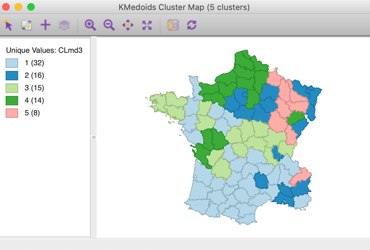
Figure 23: K Medoids CLARANS cluster map (k=5)

The cluster medoids listed in Figure 24 show all different cluster centers under CLARANS, except for CL5 (which is essentially unchanged). The total within sum of distances is 301.177, quite a bit larger than 265.147 for PAM. Correspondingly, the ratio of within to total is much higher as well, at 0.756.

CLARANS is a large data method and is optimized for speed (especially with large n and large k). It should not be used in smaller samples, where the exhaustive search carried out by PAM can be computed in a reasonable time.

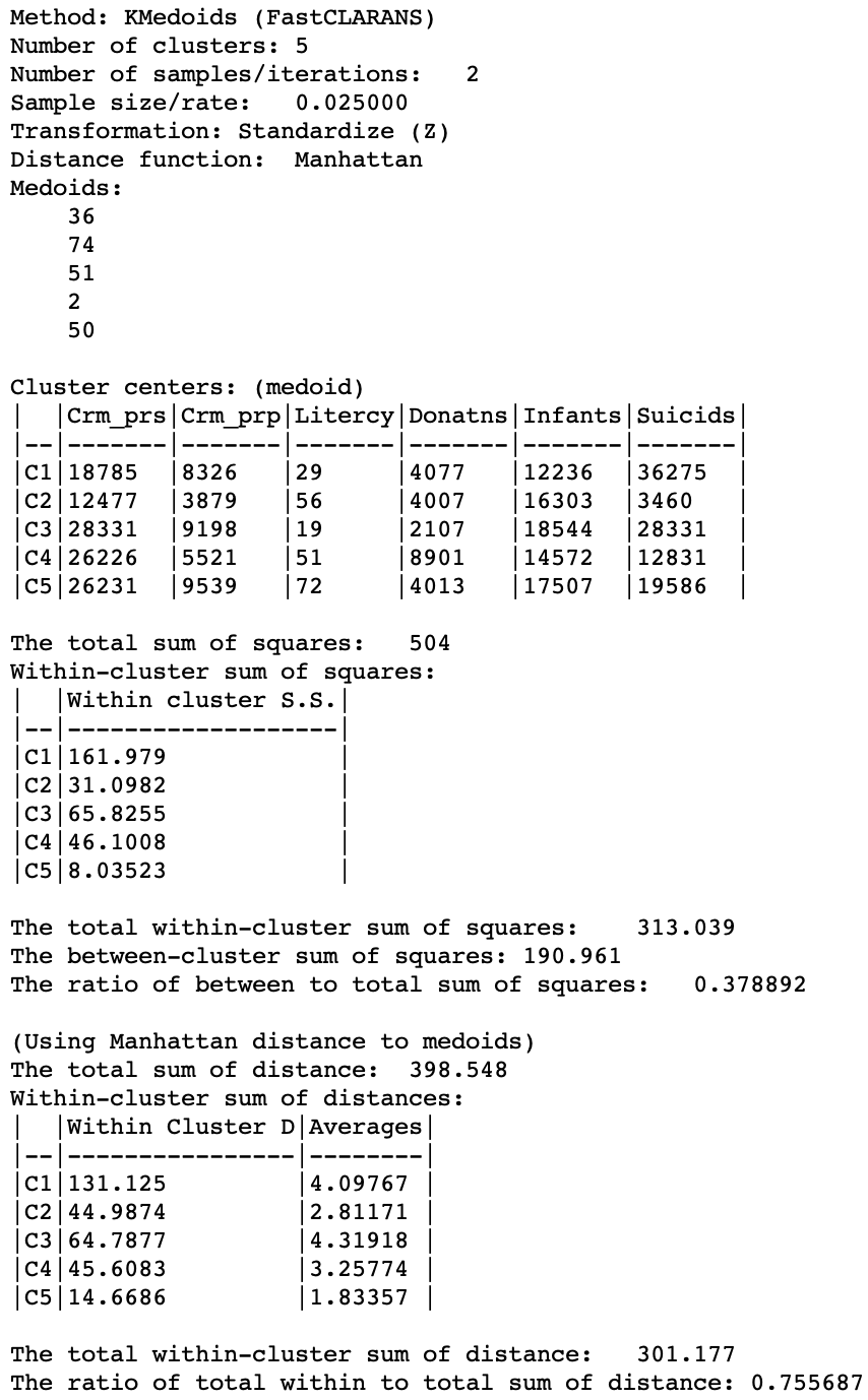
Figure 24: K Medoids CLARANS cluster characteristics (k=5)

Comparison of methods and initialization settings

In order to provide a better idea of the various trade-offs involved in the selection of algorithms and initialization settings, Figures 25 and 26 list the results of a number of experiments, for different values of k and n.

Figure 25 pertains to a sample of 791 Chicago census tracts and a clustering of socio-economic characteristics that were reduced to 5 principal components.¹⁰ For this number of observations, computation time is irrelevant, since all results are obtained almost instantaneously (in less than a second).

The number of clusters is considered for k = 5, 10, 30, 77 (the number of community areas in the city), and 150. Recall that the value of k is a critical component of the sample size for CLARA (80 + 2k) and CLARANS (a percentage of \(k \times (n-k)\)). In all cases, PAM with LAB obtains the best local minimum (for k=5, it is tied with PAM-BUILD). Also, CLARANS consistently gives the worst result. The gap with the best local optimum grows as k gets larger, from about 6% larger for k=5 to more than 20% for k=150. The results for CLARA are always in the middle, with LAB superior for k=5 and 10, and BUILD superior in the other instances.

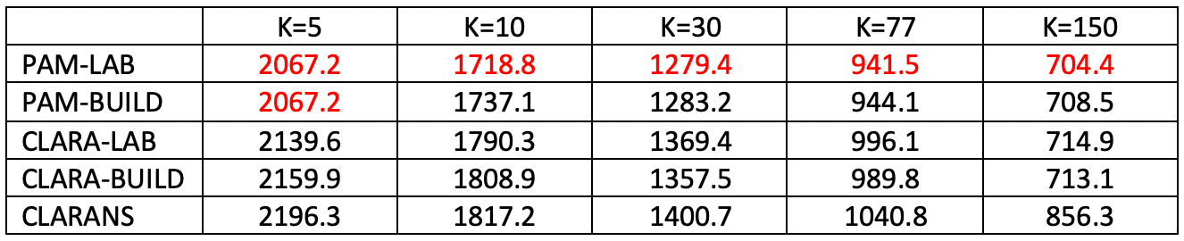
Figure 25: Local Optima - Chicago Census Tracts (n=791)

Figure 26 uses the natregimes sample data set with 3085 observations for U.S. counties. The number of variables to be clustered was increased to 20, consisting of the variables RD, PS, UE, DV and MA in all four years.

In this instance, compute time does matter, and significantly so starting with k=30. CLARANS is always the fastest, from instantaneous at k=30 to 1 second for k=300 and 2 seconds for k=500. PAM is also reasonable, but quite a bit slower, with the LAB option always faster than BUILD. For k=30, the difference between the two is minimal (2 seconds vs 3 seconds), but for k=300 PAM-LAB is about twice as fast (12 seconds vs 26 seconds), and for k=500 almost four times as fast (14 seconds vs 41 seconds). The compute time for CLARA is problematic, especially when using BUILD and for k=300 and 500 (for smaller k, it is on a par with PAM). For k=500, CLARA-BUILD takes some 6 minutes, whereas CLARA-LAB only take somewhat over a minute.

The best local optimum is again obtained for PAM, with BUILD slightly better for k=10 and 30, whereas for the other cases the LAB option is superior. In contrast to the Chicago example, CLARANS is not always worst and is better than CLARA for k = 5, 10 and 30, but not for k = 300 and 500.

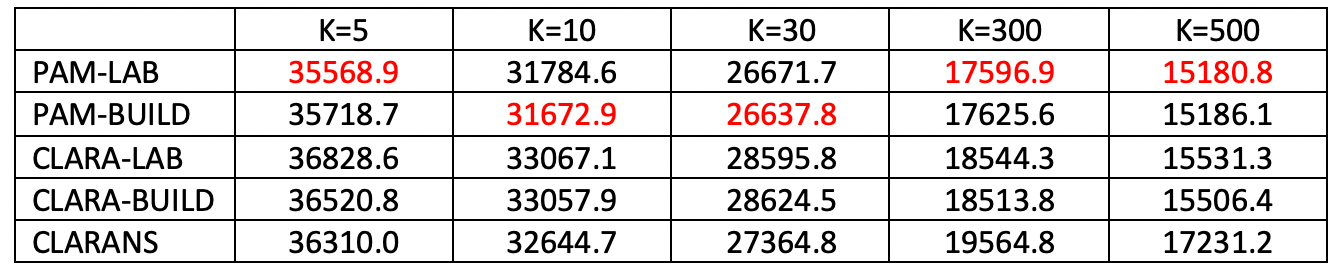
Figure 26: Local Optima - U.S. Counties (n=3085)

Overall, it seems that the FastPAM approach with the default setting of LAB performs very reliably and with decent (to superior) computation times. However, it remains a good idea to carry out further sensitivity analysis. Also, the algorithms only obtain local optima, and there is no guarantee of a global optimum. Therefore, if there is the opportunity to explore different options, they should be investigated.

Spectral Clustering

Principle

Clustering methods like k-means, k-medians or k-medoids are designed to discover convex clusters in the multidimensional data cloud. However, several interesting cluster shapes are not convex, such as the classic textbook spirals or moons example, or the famous Swiss roll and similar lower dimensional shapes embedded in a higher dimensional space. These problems are characterized by a property that projections of the data points onto the original orthogonal coordinate axes (e.g., the x, y, z, etc. axes) do not create good separations. Spectral clustering approaches this issue by reprojecting the observations onto a new axes system and carrying out the clustering on the projected data points. Technically, this will boil down to the use of eigenvalues and eigenvectors, hence the designation as spectral clustering (recall the spectral decomposition of a matrix discussed in the chapter on principal components).

To illustrate the problem, consider the result of k-means and k-medoids (for k=2) applied to the famous spirals data set from Figure 2. As Figure 27 shows, these methods tend to yield convex clusters, which fail to detect the nonlinear arrangement of the data. The k-means clusters are arranged above and below a diagonal, whereas the k-medoids result shows more of a left-right pattern.

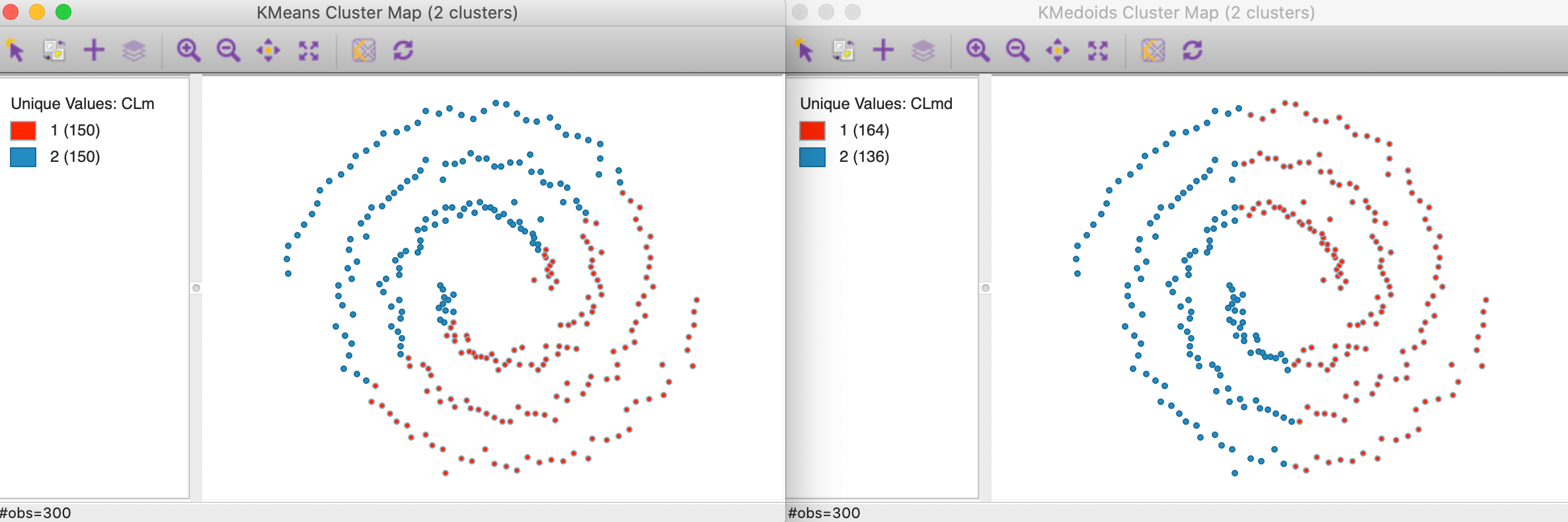
Figure 27: K-means and K-medoids on spirals data set (k=2)

In constrast, as shown in Figure 28, a spectral clustering algorithm applied to this data set perfectly extracts the two underlying patterns (initialized with a knn parameter of 3, see below for further details and illustration).

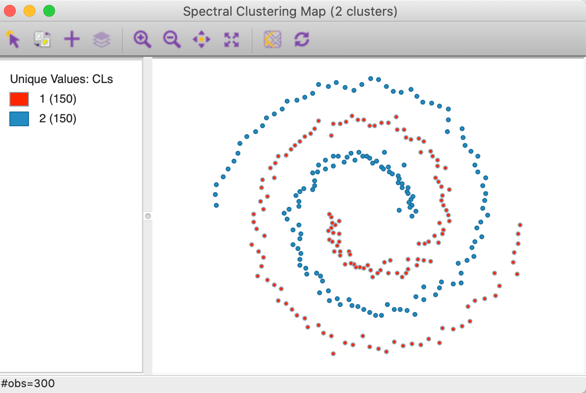
Figure 28: Spectral clustering on spirals data set (k=2)

The mathematics underlying spectral clustering view it as a problem of graph partitioning, i.e., separating a graph into subgraphs that are internally well connected, but only weakly connected with the other subgraphs. We briefly discuss this idea first, followed by an overview of the main steps in a spectral clustering algorithm, including a review of some important parameters that need to be tuned in practice.

An exhaustive overview of the various mathematical properties associated with spectral clustering is contained in the tutorial by von Luxburg (2007), to which we refer for technical details. An intuitive description is also given in Han, Kamber, and Pei (2012), pp. 519-522.

Clustering as a graph partitioning problem

So far, the clustering methods we have discussed were based on a dissimilarity matrix and had the objective of minimizing within-cluster dissimilarity. In spectral clustering, the focus is on the complement, i.e., a similarity matrix, and the goal is to maximize the internal similarity within a cluster. Of course, any dissimilarity matrix can be turned into a similarity matrix using a number of different methods, such as the use of a distance decay function (inverse distance, negative exponential) or by simply taking the difference from the maximum (e.g., \(d_{max} - d_{ij}\)).

A similarity matrix \(S\) consisting of elements \(s_{ij}\) can be viewed as the basis for the adjacency matrix of a weighted undirected graph \(G = (V,E)\). In this graph, the vertices \(V\) are the observations and the edges \(E\) give the strength of the similarity between \(i\) and \(j\), \(s_{ij}\). This is identical to the interpretation of a spatial weights matrix that we have seen before. In fact, the standard notation for the adjacency matrix is to use \(W\), just as we did for spatial weights.

Note that, in practice, the adjacency matrix is typically not the same as the full similarity matrix, but follows from a transformation of the latter to a sparse form (see below for specifics).

The goal of graph partitioning is to delineate subgraphs that are internally strongly connected, but only weakly connected with the other subgraphs. In the ideal case, the subgraphs are so-called connected components, in that their elements are all internally connected, but there are no connections to the other subgraphs. In practice, this will rarely be the case. The objective thus becomes one of finding a set of cuts in the graph that create a partioning of \(k\) subsets to maximize internal connectivity and minimize in-between connectivity. A naive application of this principle would lead to the least connected vertices to become singletons (similar to what we found in single and average linkage hierarchical clustering) and all the rest to form one large cluster. Better suited partitioning methods include a weighting of the cluster size so as to end up with well-balanced subset.¹¹

A very important concept in this regard is the graph Laplacian associated with the adjacency matrix \(W\). We discuss this further in the Appendix.

The spectral clustering algorithm

In general terms, a spectral clustering algorithm consists of four phases:

• turning the similarity matrix into an adjacency matrix

• computing the \(k\) smallest eigenvalues and eigenvectors of the graph Laplacian (alternatively, the \(k\) largest eigenvalues and eigenvectors of the affinity matrix can be calculated)

• using the (rescaled) resulting eigenvectors to carry out k-means clustering

• associating the resulting clusters back to the original observations

The most important step is the construction of the adjacency matrix, which we consider first.

Creating an adjacency matrix

The first phase consists of selecting a criterion to turn the dense similarity matrix into a sparse adjacency matrix, sometimes also referred to as the affinity matrix. The logic is very similar to that of creating spatial weights by means of a distance criterion.

For example, we could use a distance band to select neighbors that are within a critical distance \(\delta\). In the spectral clustering literature, this is referred to as an epsilon (\(\epsilon\)) criterion. This approach shares the same issues as in the spatial case when the observations are distributed with very different densities. In order to avoid isolates, a max-min nearest neighbor distance needs to be selected, which can result in a very unbalanced adjacency matrix. An adjacency matrix derived from the \(\epsilon\) criterion is typically used in unweighted form.

A preferred approach is to use k nearest neighbors, although this is not a symmetric property. Consequently, the resulting adjacency matrix is for a directed graph, since \(i\) being one of the k nearest neighbors of \(j\) does not guarantee that \(j\) is one of the k nearest neighbors for \(i\). We can illustrate this with our toy example, using two nearest neighbors for observations 5 and 6 in Figure 29. In the left hand panel, the two neighbors of observation 5 are shown as 4 and 7. In the right hand panel, 5 and 7 are neighbors of 6. So, while 5 is a neighbor of 6, the reverse is not true, creating an asymmetry in the affinity matrix (the same is true for 2 and 3: 3 is a neighbor of 2, but 2 is not a neighbor of 3).

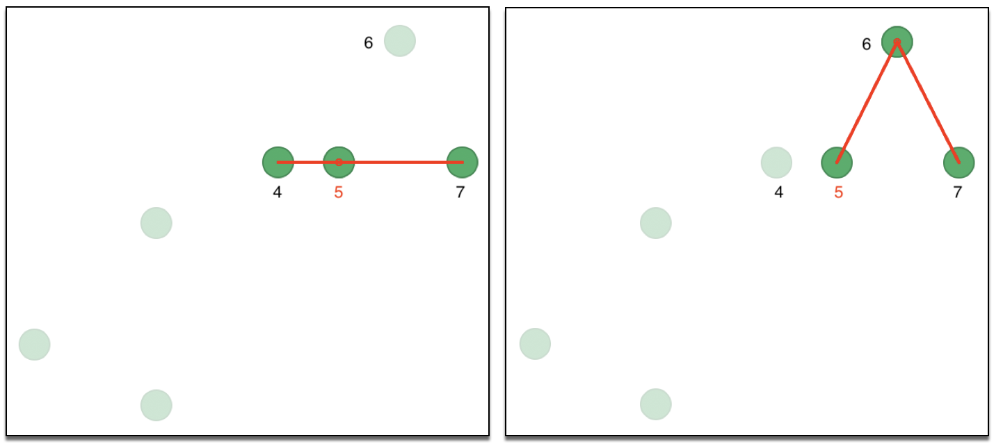
Figure 29: Asymmetry of nearest neighbors

Since the eigenvalue computations require a symmetric matrix, there are two approaches to remedy the asymmetry. In one, the affinity matrix is made symmetric as \((1/2) (W + W')\). In other words, if \(w_{ij} = 1\), but \(w_{ji} = 0\) (or the reverse), a new set of weights is created with \(w_{ij} = w_{ji} = 1/2\). This is illustrated in the left-hand panel of Figure 30, where the associated symmetric connectivity graph is shown.

Instead of a pure k-nearest neighbor criterion, so-called mutual k nearest neighbors can be defined, which consists of those neighbors among the k-nearest neighbor set that \(i\) and \(j\) have in common. More precisely, only those connectivities are kept for which \(w_{ij} = w_{ji} = 1\). The corresponding connectivity graph for our example is shown in the right hand panel of Figure 30. The links between 2 and 3 as well as between 5 and 6 have been removed.

Once the affinity matrix has been turned into a symmetric form, the resulting adjacencies are weighted with the original \(s_{ij}\) values.

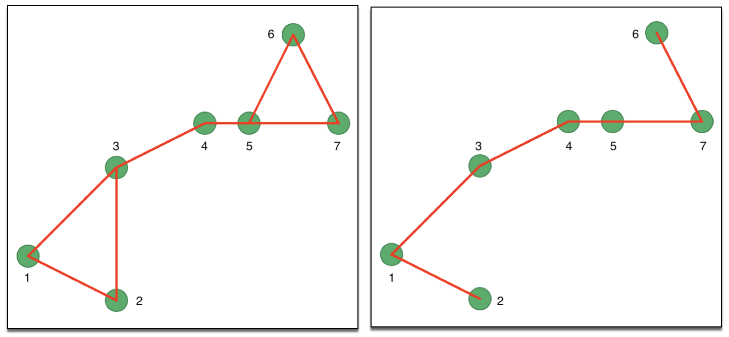
Figure 30: Symmetric k-nearest neighbor matrices

The knn adjacency matrix can join points in disconnected parts of the graph, whereas the mutual k nearest neighbors will be sparser and tends to connect observations in regions with constant density. Each has pros and cons, depending on the underlying structure of the data.

A final approach is to compute a similarity matrix that has a built-in distance decay. The most common method is to use a Gaussian density (or kernel) applied to the Euclidean distance between observations: \[s_{ij} = \exp [- (x_i - x_j)^2 / 2\sigma^2],\] where the standard deviation \(\sigma\) plays the role of a bandwidth. With the right choice of \(\sigma\), we can make the corresponding adjacency matrix more or less sparse.

Note that, in fact, the Gaussian transformation translates a dissimilarity matrix (Euclidean distances) into a similarity matrix. The new similarity matrix plays the role of the adjacency matrix in the remainder of the algorithm.

Clustering on the eigenvectors of the graph Laplacian

With the adjacency matrix in place, the \(k\) smallest eigenvalues and associated eigenvectors of the normalized graph Laplacian can be computed. Since we only need a few eigenvalues, specialized algorithms are used that only extract the smallest or largest eigenvalues/eigenvectors.¹²

When a symmetric normalized graph Laplacian is used, the \(n \times k\) matrix of eigenvectors, say \(U\), is row-standardized such that the norm of each row equals 1. The new matrix \(T\) has elements:¹³ \[t_{ij} = \frac{u_{ij}}{(\sum_{h=1}^k u_{ih}^2)^{1/2}}.\]

The new “observations” consist of the values of \(t_{ij}\) for each \(i\). These values are used in a standard k-means clustering algorithm to yield \(k\) clusters. Finally, the labels for the clusters are associated with the original observations and several cluster characteristics can be computed.

In GeoDa, the symmetric normalized adjacency matrix is used, porting to C++ the algorithm of Ng, Jordan, and Weiss (2002) as implemented in Python in scikit-learn.

Spectral clustering parameters

In practice, the results of spectral clustering tend to be highly sensitive to the choice of the parameters that are used to define the adjacency matrix. For example, when using k-nearest neighbors, the choice of the number of neighbors is an important decision. In the literature, a value of \(k\) (neighbors, not clusters) of the order of \(\log(n)\) is suggested for large \(n\) (von Luxburg 2007). In practice, both \(\ln(n)\) as well as \(\log_{10}(n)\) are used. GeoDa provides both as options.¹⁴

Simlarly, the bandwidth of the Gaussian transformation is determined by the value for the standard deviation, \(\sigma\). One suggestion for the value of \(\sigma\) is to take the mean distance to the k nearest neighbor, or \(\sigma \sim \log(n) + 1\) (von Luxburg 2007). Again, either \(\ln(n) + 1\) or \(\log_{10}(n) + 1\) can be implemented. In addition, the default value used in the scikit-learn implementation suggests \(\sigma = \sqrt{1/p}\), where \(p\) is the number of variables (features) used. GeoDa includes all three options.

In practice, these parameters are best set by trial and error, and a careful sensitivity analysis is in order.

Implementation

Spectral clustering is invoked from the Clusters toolbar, as the next to last item in the classic clustering subset, as shown in Figure 31. Alternatively, from the menu, it is selected as Clusters > Spectral.

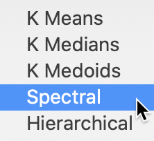
Figure 31: Spectral Clustering Option

We use the spirals data set, with an associated variable settings panel that only contains the variables x and y, as shown in Figure 32.

Variable Settings Panel

The variable settings panel has the same general layout as for the other clustering methods. One distinction is that there are two sets of parameters. One set pertains to the construction of the Affinity (or adjacency) matrix, the others are relevant for the k-means algorithm that is applied to the transformed eigenvectors. The k-means options are the standard ones.

The Affinity option provides three alternatives, K-NN, Mutual K-NN and Gaussian, with specific parameters for each. For now, we set the number of clusters to 2 and keep all options to the default setting. This includes K-NN with 3 neighbors for the affinity matrix, and all the default settings for k-means. The value of 3 for knn corresponds to \(\log_{10}(300) = 2.48\), rounded up to the next integer.

We save the cluster in the field CLs1.

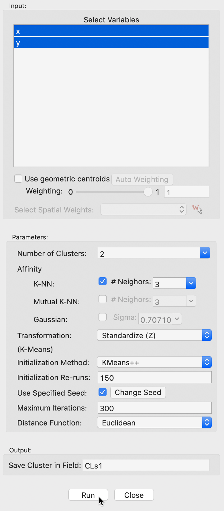
Figure 32: Spectral clustering variable selection

Cluster results

The cluster map in Figure 33 shows a perfect separation of the two spirals, with 150 observations each. As mentioned earlier, neither k-means nor k-medoids is able to extract these highly nonlinear and non-convex clusters.

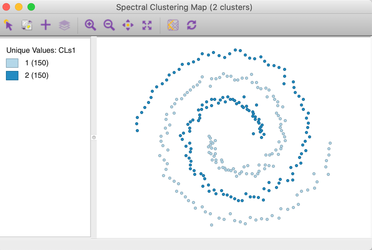
Figure 33: Spectral cluster map (k=2)

The cluster characteristics in Figure 34 list the parameter settings first, followed by the values for the cluster centers (the mean) for the two (standardized) coordinates and the decomposition of the sum of squares. The ratio of between sum of squares to total sum of squares is a dismal 0.04. This is not surprising, since this criterion provides a measure of the degree of compactness for the cluster, which a non-convex cluster like the spirals example does not meet.

In this example, it is easy to visually assess the extent to which the nonlinearity is captured. However, in the typical high-dimensional application, this will be much more of a challenge, since the usual measures of compactness may not be informative. A careful inspection of the distribution of the different variables across the observations in each cluster is therefore in order.

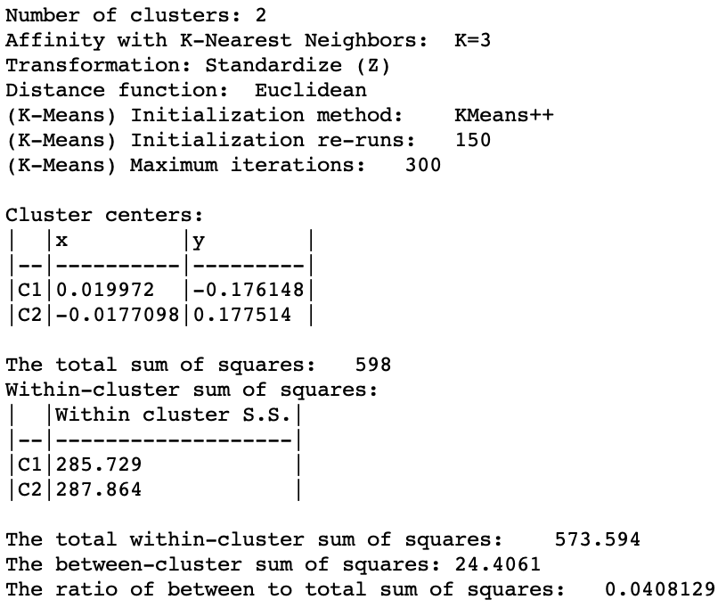
Figure 34: Spectral cluster characteristics (k=2)

Options and sensitivity analysis

The results of spectral clustering are extremely sensitive to the parameters chosen to create the affinity matrix. Suggestions for default values are only suggestions, and the particular values many sometimes be totally unsuitable. Experimentation is therefor a necessity. There are two classes of parameters. One set pertains to the number of nearest neighbors for knn or mutual knn. The other set relates to the bandwidth of the Gaussian kernel, determined by the standard deviation sigma.

K-nearest neighbors affinity matrix

The two default values for the number of nearest neighbors are contained in a drop-down list, as shown in Figure 35. In our example, with n=300, \(\log_{10}(n) = 2.48\), which rounds up to 3, and \(\ln(n) = 5.70\), which rounds up to 6. These are the two default values provided. Any other value can be entered manually in the dialog as well.

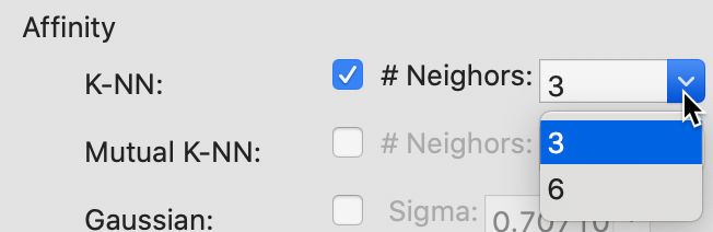
Figure 35: KNN affinity parameter values

The cluster map with knn = 6 is shown in Figure 36. Unlike what we found for the default option, this value is not able to yield a clean separation of the spirals. In addition, the resulting clusters are highly unbalanced, with respectively 241 and 59 members.

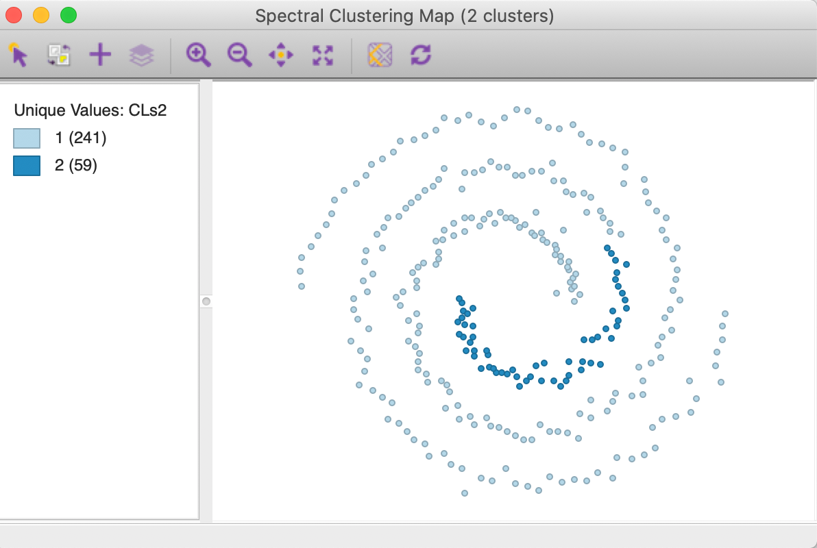
Figure 36: KNN affinity k=6 cluster map

The options for a mutual knn affinity matrix have the same entries, as in Figure 37.

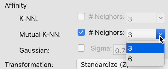
Figure 37: Mutual KNN affinity parameter values

Here again, neither of the options yields a satisfactory solution, as illustrated in Figure 38, for knn=3 in the left panel and knn=6 in the right panel. The first solution has members in both spirals, whereas the second solution does not cross over, but it only picks up part of the separate spiral.

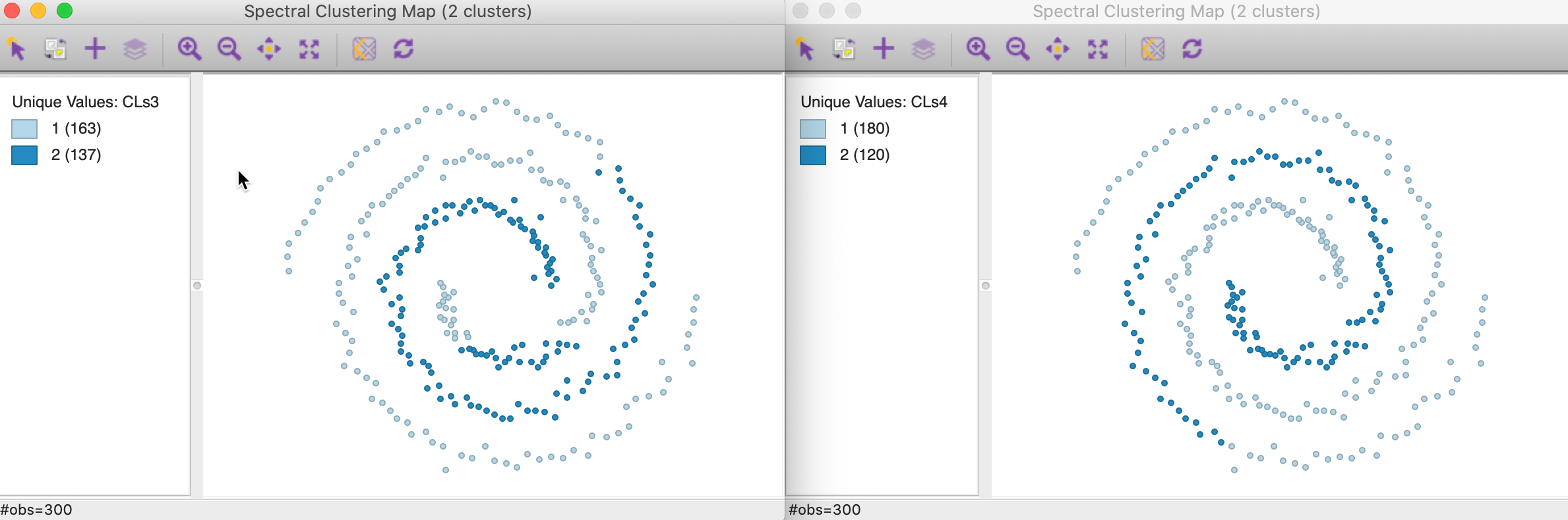
Figure 38: Mutual KNN affinity cluster maps

Gaussian kernel affinity matrix

The built-in options for sigma, the standard deviation of the Gaussian kernel are listed in Figure 39. The smallest value of 0.707107 corresponds to \(\sqrt{1/p}\), where \(p\), the number of variables, equals 2 in our example. The other two values are \(\log_{10}(n) + 1\) and \(\ln(n) + 1\), yielding respectively 3.477121 and 6.703782 for n=300. In addition, any other value can be entered in the dialog.

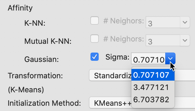
Figure 39: Gaussian kernel affinity parameter values

None of the default values yield particularly good results, as illustrated in Figure 40. In the left hand panel, the clusters are shown with \(\sigma = 0.707107\). The result totally fails to extract the shape of the separate spirals and looks similar to the results for k-mean and k-median in Figure 27. The result for \(\sigma = 6.703782\) is almost identical, with the roles of cluster 1 and 2 switched. Both are perfectly balanced clusters (the result for \(\sigma = 3.477121\) are similar).

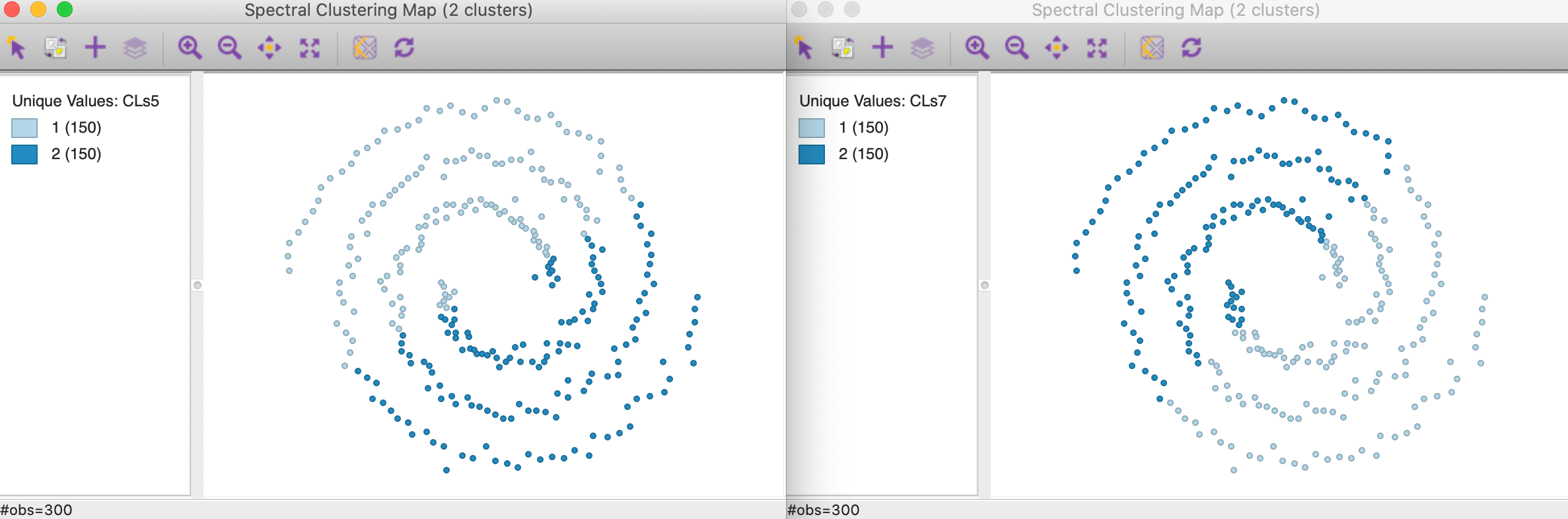
Figure 40: Gaussian kernel affinity cluster maps

In order to find a solution that provides the same separation as in Figure 33, we need to experiment with different values for \(\sigma\). As it turns out, we obtain the same result as for knn with 3 neighbors for \(\sigma = 0.08\) or \(0.07\), neither of which are even close to the default values. This illustrates how in an actual example, where the results cannot be readily visualized in two dimensions, it may be very difficult to find the parameter values that discover the true underlying patterns.

Appendix

Worked example for k-medians

We use the same toy example as in the previous chapters to illustrate the workings of the k-median algorithm. For easy reference, the coordinates of the seven points are listed again in the second and third columns of Figure 41.

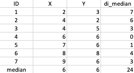
Figure 41: Worked example - basic data

The corresponding dissimilarity matrix is based on the Manhattan distance metric, i.e., the sum of the absolute difference in the x and y coordinates between the points. The result is given in Figure 42.

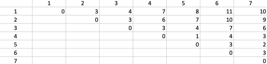
Figure 42: Manhattan distance matrix

The median center of the data cloud consists of the median of the x and y coordinates. In our case, this is the point (6,6), as shown in Figure 41. This happens to coincide with one of the observations (4), but in general this would not be the case. The distances from each observation to the median center are listed in the fourth column of 41. The sum of these distances (24) can be used to gauge the improvement that follows from each subsequent cluster allocation.

As in the k-means algorithm, the first step consists of randomly selecting k starting centers. In our example, with k=2, we select observations 4 and 7, as we did for k-means. Figure 43 gives the Manhattan distance between each observation and each of the centers. Observations closest to the respective center are grouped into the two initial clusters. In our example, these first two clusters consist of 1, 2, 3, and 5 assigned to center 4, and 6 assigned to center 7.

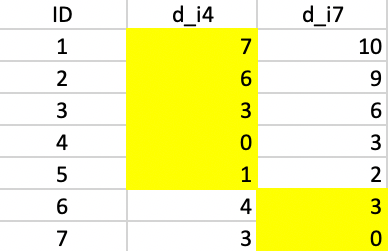
Figure 43: K-median - step 1

Next, we calculate the new cluster medians and compute the total within cluster distance as the sum of the distances from each allocated observation to the median center. This is illustrated in Figure 44. For the first cluster, the median is (4,5) and the total within cluster distance is 14. In the second cluster, the median is (8.5,7) and the total is 3 (in the case of an even number of observations in the cluster, the midpoint between the two values closest to the median is chosen, hence 8.5 and 7). The value of the objective function after this first step is thus 14 + 3 = 17.

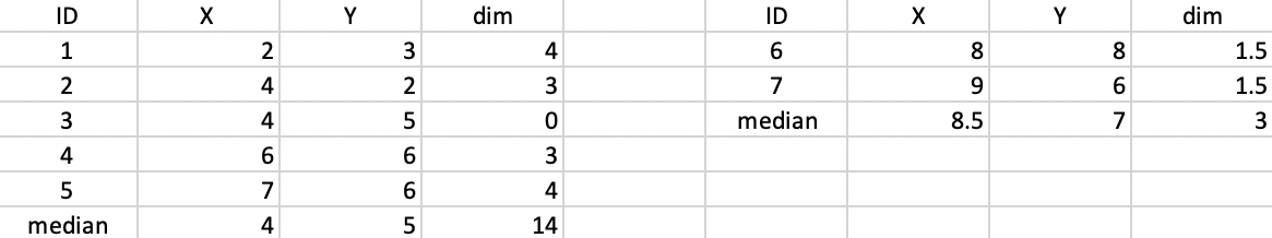
Figure 44: K-median - step 1 distance to median

We repeat the procedure, calculate the distance from each observation to both cluster centers and assign the observation to the closest center. This results in observation 5 moving from cluster 1 to cluster 2, as illustrated in Figure 45.

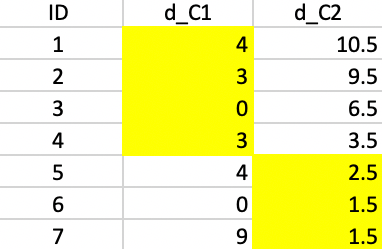
Figure 45: K-median - step 2

The new allocation results in (4,3.5) as the median center for the first cluster, and (8,6) as the center for the second cluster, as shown in Figure 46. The total distance decreases to 10 + 4 = 14.

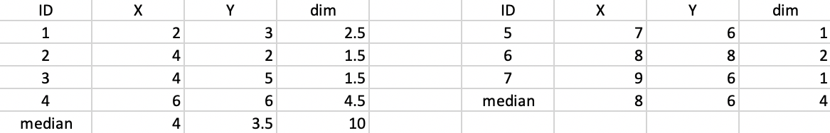
Figure 46: K-median - step 2 distance to median

We compute the distances to the two new centers in Figure 47 and assign the observations to the closest center. Now, observation 4 moves from the first cluster to the second cluster.

Figure 47: K-median - step 3

The updated median centers are (4,3) and (7.5,6) as shown in Figure 48. The total distance is 5 + 6 = 11.

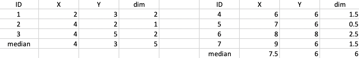
Figure 48: K-median - step 3 distance to median

Finally, computing the distances to the new centers does not induce any more changes, and the algorithm concludes (Figure 49).

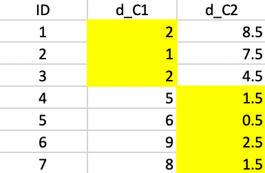
Figure 49: K-median - final allocation

The first cluster consists of 1, 2, and 3 with a median center of (4,3), the second cluster consists of 4, 5, 6, and 7 with a median center of (7.5,6). Neither of these are actual observations. The clustering resulted in a reduction of the total sum of distances to the center from 24 to 11.

The ratio 11/24 = 0.458 gives a measure of the relative improvement of the objective function. It should not be confused with the ratio of within sum of squares to total sum of squares, since the latter uses a different measure of fit (squared differences instead of absolute differences) and a different reference point (the mean of the cluster rather than the median). So, the two measures are not comparable.

Worked example for PAM

We continue to use the same toy example, with the point coordinates as in Figure 41 and associated Manhattan distance matrix in Figure 42.

BUILD

In the BUILD phase, since \(k=2\), we need find two starting centers. The first center is the observation that minimizes the row or column sum of the Manhattan distance matrix. In Figure 41, we saw that the median center coincided with observation 4 (6,6), with an associated sum of distances to the center of 24. That is our point of departure. To find the second center, we need for each candidate (i.e., the 6 remaining observations) the distance to observation 4, the current closest center (there is only one, so that is straightforward in our example). The associated values are listed below the observation ID in the second row of Figure 50.

Next, we evaluate for each row-column combination \(i,j\) the expression \(\mbox{max}(d_{j4} - d_{ij},0)\), and enter that in the corresponding element of the matrix. For example, for column 1 and row 2, that value is \(7 - d_{2,1} = 7 - 3 = 4\). For column 1 and row 5, the corresponding value is \(7 - 8 = -1\), which results in a zero entry.

With all the values entered in the matrix, we compute the row sums. There is a tie between observations 3 and 7. For consistency with our other examples, we pick 7 as the second starting point.

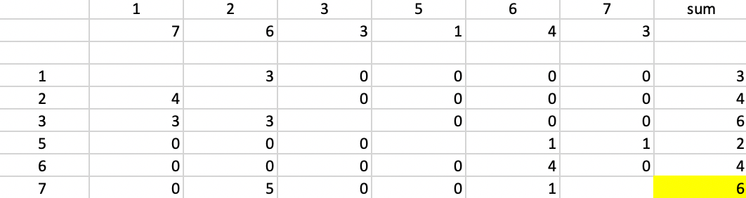
Figure 50: PAM - finding the second initial center

SWAP

The initial stage is the same as for the k-median example, given in Figure 43. The total distance to each cluster center equals 20, with cluster 1 contributing 17 and cluster 2, 3.

The first step in the swap procedure consists of evaluating whether center 4 or center 7 can be replaced by any of the current non-centers, i.e., 1, 2, 3, 5, or 6. The comparison involves three distances for each point: the distance to the closest center, the distance to the second closest center, and the distance to the candidate center. In our example, this is greatly simplified, since there are only two centers, with distances \(d_{j4}\) and \(d_{j7}\) for each non-candidate and non-center point \(j\). In addition, we need the distance to the candidate center \(d_{jr}\), where each non-center point is in turn considered as a candidate (\(r\) in our notation).

All the evaluations for the first step are included in Figure 51. There are five main panels, one for each current non-center point. The rows in each panel are the non-center, non-candidate points. For example, in the top panel, 1 is considered a candidate, so the rows pertain to 2, 3, 5, and 6. Columns 3-4 give the distance to, respectively, center 4 (\(d_{j4}\)), center 7 (\(d_{j7}\)) and candidate center 1 (\(d_{j1}\)).

Columns 5 and 6 give the contribution of each row to the objective with point 1 replacing, respectively 4 (\(C_{j41}\)) and 7 (\(C_{j71}\)). First consider a replacement of 4 by 1. For point 2, the distances to 4 and 7 are 6 and 9, so point 2 is closest to center 4. As a result 2 will be allocated to either the new candidate center 1 or the current center 7. It is closest to the new center (3 relative to 9). The decrease in the objective from assigning 2 to 1 rather than 4 is 3 - 6 = -3, the entry in the column \(C_{j41}\).

Now consider the contribution of 2 to the replacement of 7 by 1. Since 2 is closer to 4, we have the situation that a point is not closest to the center that is to be replaced. So, now we need to check whether it would stay with its current center (4) or move to the candidate. We already know that 2 is closer to 1 than to 4, so the gain from the swap is again -3, entered under \(C_{j71}\). We proceed in the same way for each of the other non-center and non-candidate points and find the sum of the contributions, listed in the row labeled \(T\). For a replacement of 4 by 1, the sum of -3, 1, 1, and 0 gives -1 as the value of \(T_{41}\). Similarly, the value of \(T_{47}\) is the sum of -3, 0, 0, and 1, or -2.

The remaining panels show the results when each of the other current non-centers is evaluated as a center candidate. The minimum value over all pairs \(i,r\) is obtained for \(T_{43} = -5\). This suggests that center 4 should be replaced by point 3 (there is actually a tie with \(T_{73}\), so in each case 3 should enter the center set; we take it to replace 4). The improvement in the overall objective function from this step is -5.

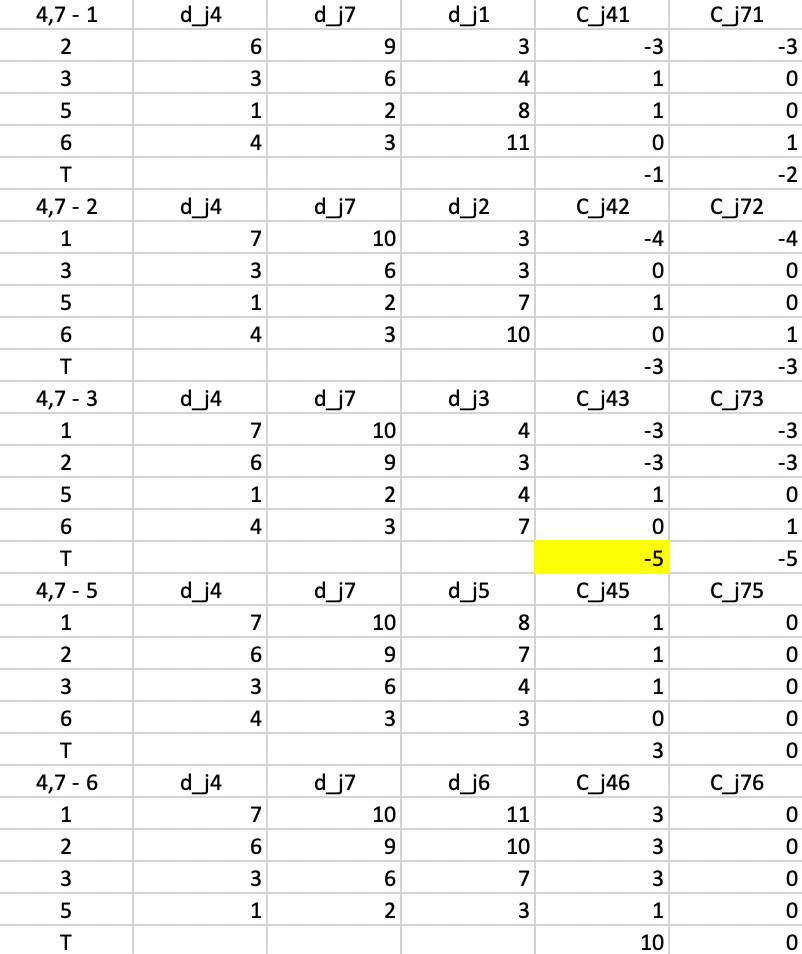
Figure 51: PAM - swap step 1

This process is repeated in Figure 52, but now using \(d_{j3}\) and \(d_{j7}\) as reference distances. The smallest value for \(T\) is found for \(T_{75} = -2\), which is also the improvement to the objective function (note that the improvement is smaller than for the first step, something we would expect from a gradient descent method). This suggests that 7 should be replaced by 5.

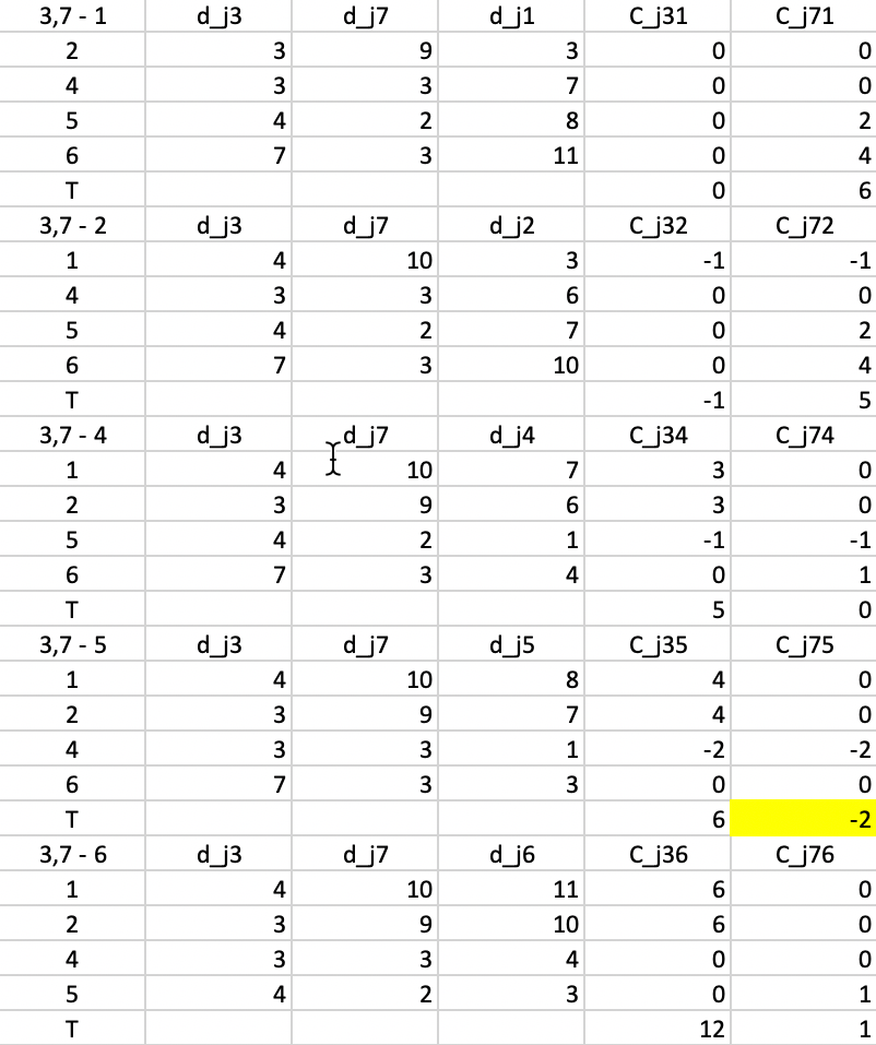
Figure 52: PAM - swap step 2

In the next step, we repeat the calculations, using \(d_{j3}\) and \(d_{j5}\) as the distances. The smallest value for \(T\) is found for \(T_{32} = -1\), suggesting that 3 should be replaced by 2. The improvement in the objective is -1 (again, smaller than in the previous step).

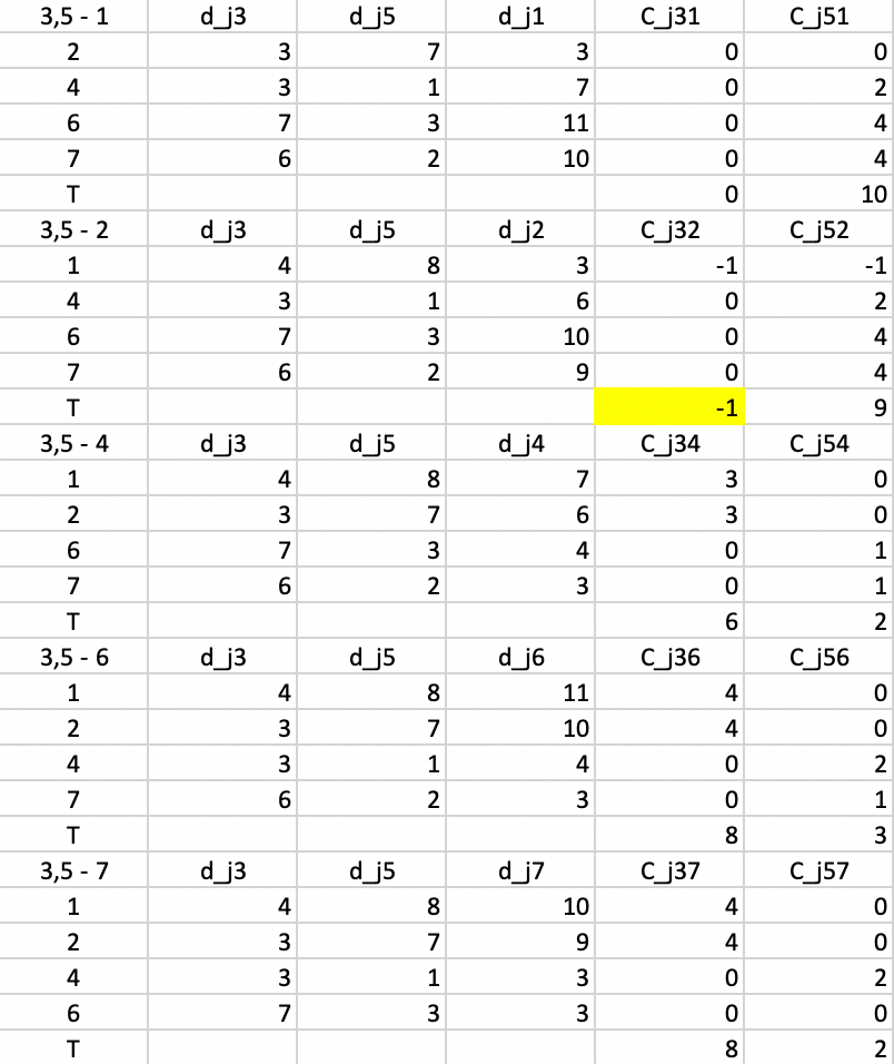
Figure 53: PAM - swap step 3

In the last step, we compute everything again for \(d_{j2}\) and \(d_{j5}\). At this stage, none of the \(T\) yield a negative value, so the algorithm has reached a local optimum and stops.

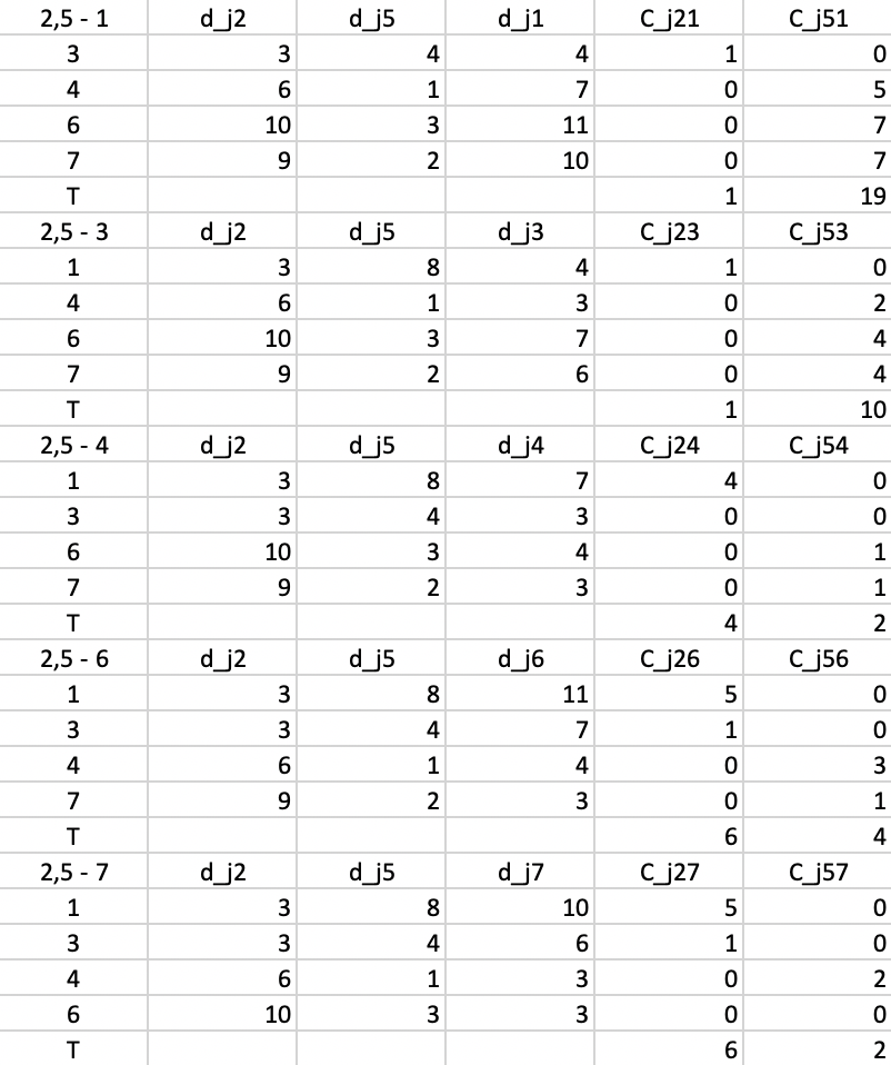
Figure 54: PAM - swap step 4

The final result consists of a cluster of three elements, centered on 2, and a cluster of four elements, centered on 5. As Figure 55 shows, both clusters contribute 6 to the total sum of deviations, for a final value of 12. This also turns out to be 20 - 5 - 2 - 1, or the total effect of each swap on the objective function.

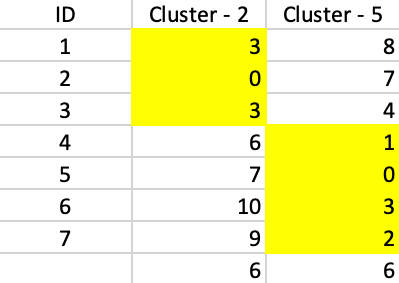
Figure 55: PAM - final solution

The graph Laplacian

A useful property of the adjancency matrix \(W\) associated with a graph is the degree of a vertex \(i\): \[d_i = \sum_j w_{ij},\] the row-sum of the similarity weights. Previously, we used an identical concept to characterize the connectivity structure of a spatial weights, and referred to it as neighbor cardinality.

The graph Laplacian is the following matrix: \[L = D - W,\] where \(D\) is a diagonal matrix containing the degree of each vertex. The graph Laplacian has the property that all its eigenvalues are real and non-negative, and, most importantly, that its smallest eigenvalue is zero.

In the (ideal) case where the adjacency matrix can be organized into separate partitions (unconnected to each other), it takes on a block-diagonal form, with each block containing the partioning sub-matrix for the matching group. The corresponding graph Laplacian will similarly have a block-diagonal structure. Since each of these sub-blocks is itself a graph Laplacian (for the subnetwork corresponding to the partition), its smallest eigenvalue is zero as well. An important result is then that if the graph is partitioned into \(k\) disconnected blocks, the graph Laplacian will have \(k\) zero eigenvalues. This forms the basis for the logic of using the \(k\) smallest eigenvalues of \(L\) to find the corresponding clusters.

While it can be used to proceed with spectral clustering, the unnormalized Laplacian \(L\) has some undesirable properties. Instead, the preferred approach is to use a so-called normalized Laplacian. There are two ways to normalize the adjacency matrix and thus the associated Laplacian. One is to row-standardize the adjacency matrix, or \(D^{-1}W\). This is exactly the same idea as row-standardizing a spatial weights matrix. When applied to the Laplacian, this yields: \[L_{rw} = D^{-1}L = D^{-1}D - D^{-1}W = I - D^{-1}W.\] This is referred to as a random walk normalized graph Laplacian, since the row elements can be viewed as transition probabilities from state \(i\) to each of the other states \(j\). As we saw with spatial weights, the resulting normalized matrix is no longer symmetric, although its eigenvalues remain real, with the smallest eigenvalue being zero. The associated eigenvector is \(\iota\), a vector of ones.

A second transformation pre- and post-multiplies the Laplacian by \(D^{-1/2}\), the inverse of the square root of the degree. This yields a symmetric normalized Laplacian as: \[L_{sym} = D^{-1/2}LD^{-1/2} = D^{-1/2}DD^{-1/2} - D^{-1/2}WD^{-1/2} = I - D^{-1/2}WD^{-1/2}.\] Again, the smallest eigenvalue is zero, but the associated eigenvector is \(D^{1/2}\iota\).

Spectral clustering algorithms differ by whether the unnormalized or normalized Laplacian is used to compute the \(k\) smallest eigenvalues and associated eigenvectors and whether the Laplacian or the adjacency matrix is the basis for the calculation.

Specifically, as an alternative to using the smallest eigenvalues and associated eigenvectors of the normalized Laplacian, the largest eigenvalues/eigenvectors of the normalized adjacency (or affinity) matrix can be computed. The standard eigenvalue expression is the following equality: \[Lu = \lambda u,\] where \(u\) is the eigenvector associated with eigenvalue \(\lambda\). If we subtract both sides from \(Iu\), we get: \[(I - L)u = (1 - \lambda)u.\] In other words, if the smallest eigenvalue of \(L\) is 0, then the largest eigenvalue of \(I - L\) is 1. Moreover: \[I - L = I - [I - D^{-1/2}WD^{-1/2}] = D^{-1/2}WD^{-1/2},\] so that the search for the smallest eigenvalue of \(L\) is equivalent to the search for the largest eigenvalue of \(D^{-1/2}WD^{-1/2}\), the normalized adjacency matrix.

References

Anselin, Luc. 2019. “Quantile Local Spatial Autocorrelation.” Letters in Spatial and Resource Sciences 12 (2): 155–66.

Han, Jiawei, Micheline Kamber, and Jian Pei. 2012. Data Mining (Third Edition). Amsterdam: MorganKaufman.

Hastie, Trevor, Robert Tibshirani, and Jerome Friedman. 2009. The Elements of Statistical Learning (2nd Edition). New York, NY: Springer.

Hoon, Michiel de, Seiya Imoto, and Satoru Miyano. 2017. “The C Clustering Library.” Tokyo, Japan: The University of Tokyo, Institute of Medical Science, Human Genome Center.

Kaufman, L., and P. Rousseeuw. 2005. Finding Groups in Data: An Introduction to Cluster Analysis. New York, NY: John Wiley.

Ng, Andrew Y., Michael I. Jordan, and Yair Weiss. 2002. “On Spectral Clustering: Analysis and an Algorithm.” In Advances in Neural Information Processing Systems 14, edited by T. G. Dietterich, S. Becker, and Z. Ghahramani, 849–56. Cambridge, MA: MIT Press.

Ng, Raymond R., and Jiawei Han. 2002. “CLARANS: A Method for Clustering Objects for Spatial Data Mining.” IEEE Transactions on Knowledge and Data Engineering 14: 1003–16.

Schubert, Erich, and Peter J. Rousseeuw. 2019. “Faster k-Medoids Clustering: Improving the PAM, CLARA, and CLARANS Algorithms.” In Similarity Search and Applications, SISAP 2019, edited by Giuseppe Amato, Claudio Gennaro, Vincent Oria, and Miloš Radovanović, 171–87. Cham, Switzerland: Springer Nature.

Shi, Jianbo, and Jitendra Malik. 2000. “Normalized Cuts and Image Segmentation.” IEEE Transactions on Pattern Analysis and Machine Intelligence 22 (8): 888–905.

von Luxburg, Ulrike. 2007. “A Tutorial on Spectral Clustering.” Statistical Computing 27 (4): 395–416.

---

1. University of Chicago, Center for Spatial Data Science – anselin@uchicago.edu↩︎

2. Strictly speaking, k-medoids minimizes the average distance to the representative center, but the sum is easier for computational reasons.↩︎

3. As Kaufman and Rousseeuw (2005) show in Chapter 2, the problem is identical to some facility location problems for which integer programming branch and bound solutions have been suggested. But these tend to be limited so smaller sized problems.↩︎

4. Clearly, with a sample size of 100%, CLARA becomes the same as PAM.↩︎

5. More precisely, the first sample consists of 40 + 2k random points. From the second sample on, the best k medoids found in a previous iteration are included, so that there are 40 + k additional random points. Also, in Schubert and Rousseeuw (2019), they suggested to use 80 + 4k and 10 repetitions for larger data sets. In the implementation in GeoDa, the latter is used for data sets larger than 100.↩︎

6. Schubert and Rousseeuw (2019) also consider 2.5% in larger data sets with 4 iterations instead of 2.↩︎

7. The Java code is contained in the open source ELKI software, available from https://elki-project.github.io.↩︎

8. This is the approach used to obtain the selections in Figure 16.↩︎

9. As mentioned, for sample sizes > 100, GeoDa uses a sample size of 80 + 4k.↩︎

10. The data set is available as one of the GeoDa Center sample data. Details about the computation of the principal components and other aspects of the data are given in Anselin (2019).↩︎

11. For details, see Shi and Malik (2000), as well as the discussion of a “graph cut point of view” in von Luxburg (2007).↩︎

12. GeoDa uses the Spectra C++ library for large scale eigenvalue problems. Note that the particular routines implemented in this library extract the largest eigenvalues/eigenvectors from the symmetric normalized affinity matrix, not the smallest from the graph Laplacian. The latter is the textbook explanation, but not always the most efficient implementation in practice. The equivalence between the two approaches is detailed in the Appendix.↩︎

13. Alternative normalizations are used as well. For example, in the implementation in scikit-learn, the eigenvectors are rescaled by the inverse square root of the eigenvalues.↩︎

14. In GeoDa, the values for the number of nearest neighbors are rounded up to the nearest integer.↩︎

GeoDa is maintained by lixun910. This page was generated by GitHub Pages using the Cayman theme by Jason Long.