Density-Based Clustering Methods

Introduction

In this chapter, we consider density based clustering methods. These approaches look in the data for high density subregions of arbitrary shape, separated by low-density regions. Alternatively, the regions can be interpreted as modes in the spatial distribution over the support of the observations.

These methods are situated in between the local spatial autocorrelation statistics and the regionalization methods we consider in later chapters. They pertain primarily to point patterns, but can also be extended to a full multivariate setting. Even though they show many similarities with spatially constrained clustering methods, they are not quite the same, in that they do not necessarily yield a complete partitioning of the data. Therefore, they are considered separately, even though they are included under the Cluster Methods in GeoDa.

Attempts to discover high density regions in the data distribution go back to the classic paper on mode analysis by Wishart (1969), and its refinement in Hartigan (1975). In the literature, these methods are also referred to as bump hunting, i.e., looking for bumps (high regions) in the data distribution.

In this chapter, we will focus on the application of density-based clustering methods to the geographic location of points, but they are generalizable to locations in high-dimensional attribute space as well.

An important concept in this respect is that of a level set associated with a given density level \(\lambda\): \[L(\lambda; p) = \{ x | p(x) \gt \lambda\},\] i.e., the collection of data points \(x\) for which the probability exceeds the given threshold. A subset of such points that contains the maximum number of points that are connected (so-called connected components) is called a density-contour cluster of the density function. A density-contour tree is then a tree formed of nested clusters that are obtained by varying the level \(\lambda\) (Hartigan 1975; Müller and Sawitzki 1991; Stuetzle and Nugent 2010).

To visualize this concept, consider the data distribution represented as a three-dimensional surface. Then, a level set consists of those data points that are above a horizontal plane at \(\lambda\), e.g., as islands sticking out of the ocean. As \(\lambda\) increases, the level set becomes smaller. In our island analogy, this corresponds to a rising ocean level (the islands become smaller and may even disappear). In the other direction, as \(\lambda\) decreases, or the ocean level goes down, connections between islands (a land bridge) may become visible so that they no longer appear separated, but rather as a single entity.

As mentioned, in contrast to the classic cluster methods discussed in later methods, density-based methods do not necessarily yield a complete regionalization, and some observations (points) may not be assigned to any cluster. In turn, some of these points can be interpreted as outliers, which is of main interest in certain applications. In a sense, the density-based cluster methods are similar in spirit to the local spatial autocorrelation statistics, although most of them are not formulated as hypothesis tests.

We consider four approaches. We begin with a simple heat map as a uniform density kernel centered on each location. The logic behind this graph is similar to that of Openshaw’s geographical analysis machine (Openshaw et al. 1987) and the approach taken in spatial scan statistics (Kulldorff 1997), i.e., a simple count of the points within the given radius.

The next methods are all related to DBSCAN (Ester et al. 1996), or Density Based Spatial Clustering of Applications with Noise. We consider both the original DBSCAN, as well as its improved version, referred to as DBSCAN*, and its Hierarchical version, referred to as HDBSCAN (or, sometimes, HDBSCAN*) (Campello, Moulavi, and Sander 2013; Campello et al. 2015).

The methods are illustrated here using the point locations of liquor stores in Chicago (in 2015), but they can pertain to other geometric forms as well, such as clustering of polygons (Sander et al. 1998). In general, they can also be applied to any set of points in multi-attribute space (i.e., non-geographical), although that use is perhaps less common.

Objectives

• Interpret the results of a uniform kernel heat map

• Understand the principles behind DBSCAN

• Set the parameters for a DBSCAN approach

• Interpret the clustering results yielded by DBSCAN

• Understand the difference between DBSCAN and DBSCAN*

• Analyze the dendrogram generated by DBSCAN*

• Understand the logic underlying HDBSCAN

• Interpret the condensed tree and clustering results yielded by HDBSCAN

• Understand soft clustering and outlier identification in HDBSCAN

GeoDa functions covered

• Map option > Heat Map
• Clusters > DBscan
• Clusters > HDBscan

Getting started

We will use the liq_Chicago shape file with 571 point locations of liquor stores in the city of Chicago during 2015. This data set is included as one of the sample data sets, named liquor stores. The point locations were scraped from Google maps and converted to the Illinois State Plane projection.

In Figure 1, the points are shown against a backdrop of the Chicago community area boundaries.²

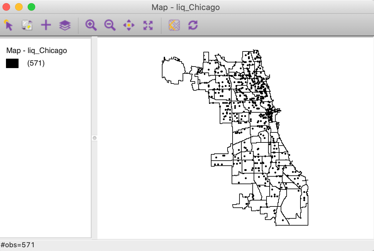
Figure 1: Chicago liquor store locations (2015)

Heat Map

Principle

The heat map as implemented in GeoDa is a simple uniform kernel for a given bandwidth. A circle with radius equal to the bandwidth is centered on each point in turn, and the number of points within the radius are counted. The density of the points is reflected in the color shading.

This is the same principle as underlying the Geographical Analysis Machine or GAM of Openshaw et al. (1987), where the uniform kernel is computed for a range of bandwidths to identify high intensity clusters. In our implementation, no significance is assigned, and the heat map is used primarily as a visual device to highlight differences in the density of the points.

Implementation

The heat map is not invoked from the cluster menu, but as an option on a point map. Right click to bring up the list of options and select Heat Map > Specify Bandwidth as in Figure 2.

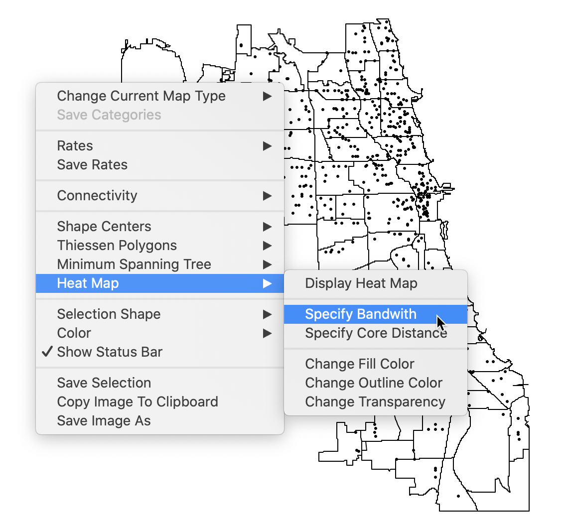
Figure 2: Specify bandwidth for heat map

This brings up the default heat map, created for a bandwidth that corresponds with the max-min distance, i.e., the largest of the nearest neighbor distances. This ensures that each point has at least one neighbor. The corresponding distance is shown in the dialog, as in Figure 3.

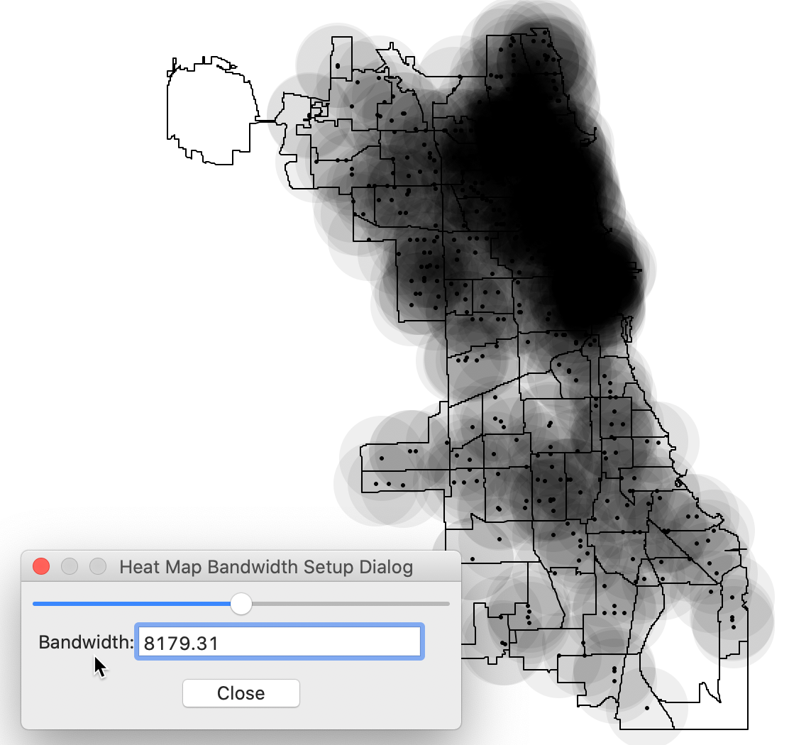
Figure 3: Default settings for heat map

The default setting is almost never very informative, especially when the points are distributed unevenly. For example, after setting the bandwidth to 3000, a much more interesting pattern is revealed, with a greater concentration of points in the near north side of the city, shown in Figure 4.

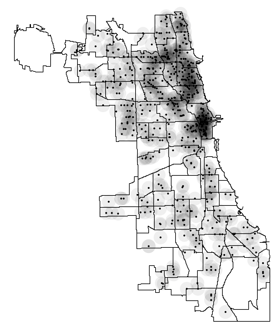
Figure 4: Heat map with bandwidth of 3000

In addition to the bandwidth, the heat map also has the option to select a variable other than the x-y coordinates to compute the kernel. This is selected in Core Distance. We do not pursue this further here.

Finally, the heat map has all the usual customization options, such as changing the fill color, the outline color, or the transparency.

DBSCAN

Principle

The DBSCAN algorithm was originally outlined in Ester et al. (1996) and Sander et al. (1998), and was more recently elaborated upon in Gan and Tao (2017) and Schubert et al. (2017). Its logic is similar to that just outlined for the uniform kernel. In essence, the method again consists of placing circles of a given radius on each point in turn, and identifying those groupings of points where a lot of locations are within each others range.

In order to quantify this, DBSCAN introduces a special terminology. Points are classified as Core, Border or Noise depending on how many other points are within a critical distance band, the so-called Eps neighborhood. To visualize this, Figure 5 contains nine points, each with a circle centered on it with radius equal to Eps.³ Note that in DBSCAN, any distance metric can be used, not just Euclidean distance as in this illustration.

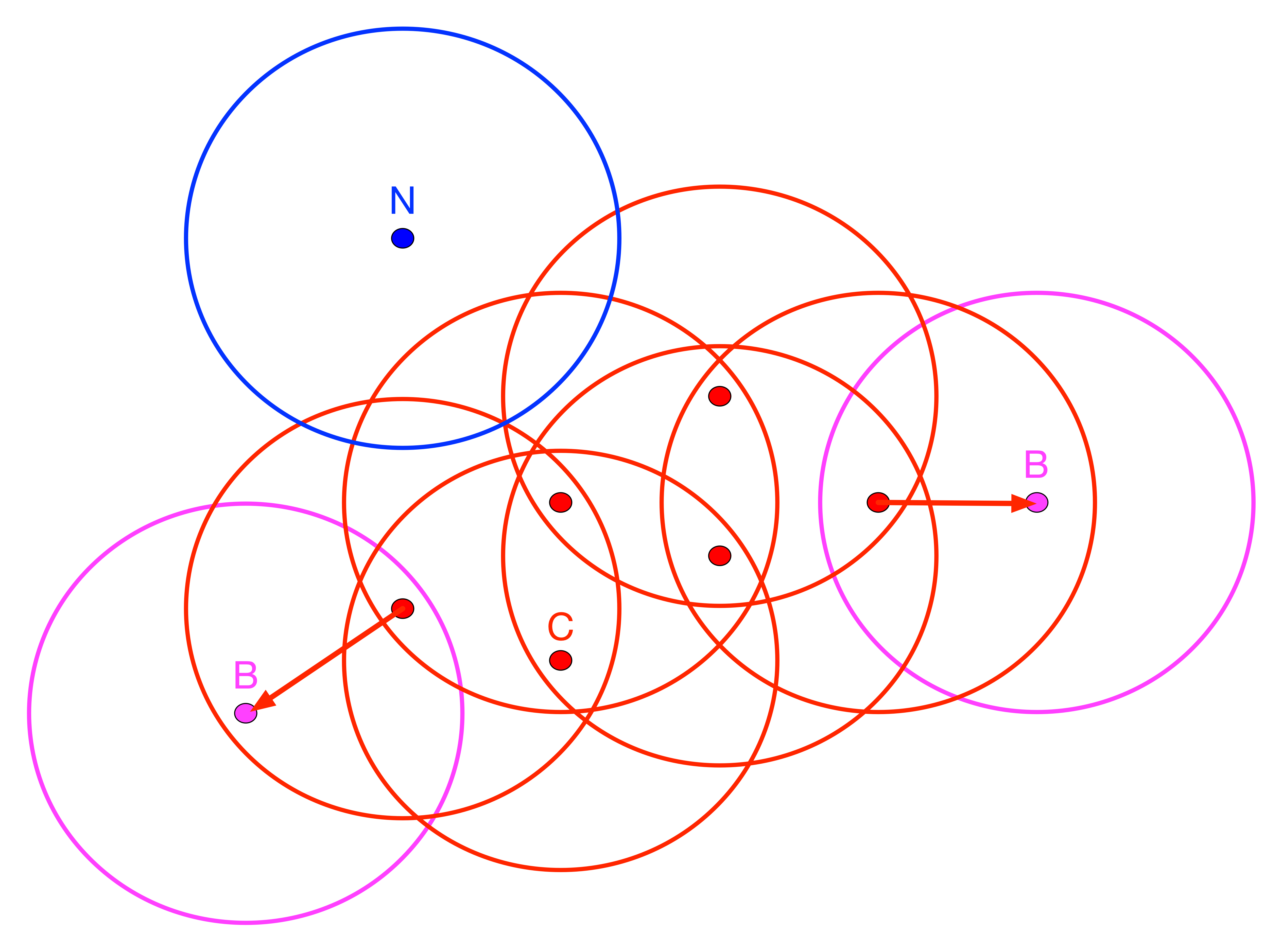
Figure 5: DBSCAN Core, Border and Noise points

A second critical concept is the number of points that need to be included in the distance band in order for the spatial distribution of points to be considered as dense. This is the so-called minimum number of points, or MinPts criterion. In our example, we take that to be four. Note, that in contrast to the convention we used before in defining k-nearest neighbors, the MinPts criterion includes the point itself. So a MinPts = 4 corresponds to a point having 3 neighbors within the Eps radius .⁴

In Figure 5, all red points with associated red circles have at least four points within the critical range (including the central point). They are labeled as Core points and are included in the cluster (point C and the other red points). The points in magenta (labeled B), with associated magenta circles have some points within the distance range (one, to be precise), but not sufficient to meet the MinPts criterion. They are potential Border points and may or may not be included in the cluster. Finally, the blue point (labeled N) with associated blue circle does not have any points within the critical range and is labeled Noise. Such a point cannot become part of any cluster.

A point is directly density reachable from another point if it belongs to the Eps neighborhood of that point and is one of MinPts neighbors of that point. This is not a symmetric relationship.

In our example, any red point is directly density reachable from at least one other red point. In turn that point is within the critical range from the original point. However, for points B, the relationship only holds in one direction, as shown by the arrow. They are directly density reachable from a red point, but since the B points only have one neighbor, their range does not meet the minimum criterion. Therefore, the neighbor is not directly density reachable from B. A chain of points in which each point is directly density reachable from the previous one is called density reachable. In order to be included, each point in the chain has to have at least MinPts neighbors and could serve as the core of a cluster. All our red points are density reachable.

In order to decide whether a border point should be included in a cluster, the concept of density connected is introduced. Two points are density connected if they are both density reachable from a third point. In our example, the points B are density connected to the other core points through their neighbor, which is itself directly density reachable from the red points in its neighborhood.

In DBSCAN, a cluster is then defined as collection of points that are density connected and maximize the density reachability. The algorithm starts by randomly selecting a point and determining whether it can be classified as Core – with at least MinPts in its Eps neighborhood – or rather as Border or Noise. A Border point can later be included in a cluster if it is density connected to another Core point. It is then assigned the cluster label of the core point and no longer further considered. One implication of this aspect of the algorithm is that once a Border point is assigned a cluster label, it cannot be assigned to a different cluster, even though it might actually be closer to the corresponding core point. In a later version, labeled DBSCAN* (considered in the next section), the notion of border points is dropped, and only Core points are considered to form clusters.

The algorithm systematically moves through all the points in the data set and repeats the process. The search for neighbors is facilitated by using an efficient spatial data structure, such as an R* tree. When two clusters are density connected, they are merged. The process continues until all points have been evaluated.

Two critical parameters in the DBSCAN algorithm are the distance range and the minimum number of neighbors. In addition, sometimes a tolerance for noise points is specified as well. The latter constitute zones of low density that are not deemed to be interesting.

In order to avoid any noise points, the critical distance must be large enough so that every point is at least density connected. An analogy is the specification of a max-min distance band in the creation of spatial weights, which ensures that each point has at least one neighbor. In practice, this is typically not desirable, but in some implementations a maximum percentage of noise points can be set to avoid too many low density areas.⁵

Ester et al. (1996) recommend that MinPts be set at 4 and the critical distance adjusted accordingly to make sure that sufficient observations can be classified as Core. As in other cluster methods, some trial and error it typically necessary. Finding a proper value for Eps is often considered a major drawback of the DBSCAN algorithm.

An illustration of the detailed steps and logic of the algorithm is provided by a worked example in the Appendix.

Implementation

DBSCAN is invoked from the cluster toolbar icon as the first item in the density cluster group, or from the menu as Clusters > DBScan , as shown in Figure 6.

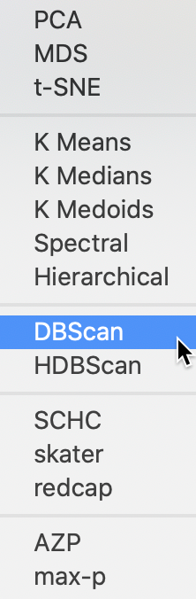
Figure 6: DBscan option

The usual cluster interface appears, listing the variables in the data table and the various parameters to be selected, as in Figure 7. In our example, we only have <X-Centroids> and <Y-Centroids>, since only the location information of the stores has been included. The default is to have the Method selected as DBScan (DBSCAN* is uses the same interface and is discussed next). In addition, we make sure that the Transformation is set to Raw, in order to use the original coordinates, without any transformations.

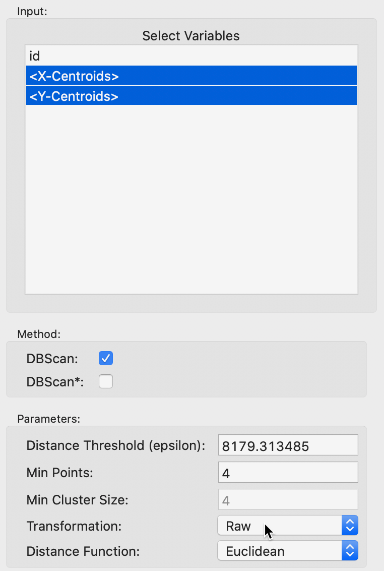
Figure 7: DBSCAN variable selection

As seen in Figure 7, the default uses the largest nearest neighbor distance of 8179 (feet) such that all observations are connected (note that this is the same distance as the default bandwidth in Figure 3). We can check in the weights manager dialog that this is indeed the distance that would be the default to create a fully connected distance band spatial weight. This yields a median number of neighbors of 30, with a minimum of 1 and a maximum of 79. Needless to say, the default Min Points value of 4 is not very meaningful in this context.

The resulting cluster map is shown in Figure 8. It contains two clusters, one very large one with 561 observations, and a small one with 7 observations. In addition, three points are classified as Noise. The Summary panel contains the usual information on cluster centers and sum of squares, which is not very relevant in this example. There is also a button for Dendrogram, which is only used for DBSCAN* and is empty in the current example.

We assess more meaningful parameter values in the next set of examples.

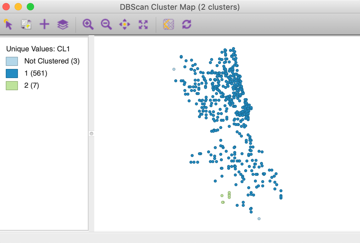
Figure 8: DBSCAN cluster map for default settings

Border points and minimum cluster size

The DBSCAN algorithm depends critically on the choice of two parameters. One is the Distance Threshold, or Eps. The other is the minimum number of neighbors within this epsilon distance band that an observation must have in order to be considered a Core point, i.e., the Min Points parameter. Each cluster must contain at least one core point.

As Eps decreases, more and more points will become disconnected and thus will be automatically categorized as Noise. For example, for a distance band of 3000 (as in the heat map in Figure 4), we can visualize the connectivity graph of the corresponding distance band spatial weights, as in Figure 9. This yields 37 unconnected points with neighbors ranging from 0 to 30, with a median of 4.

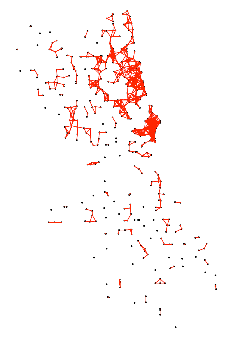
Figure 9: Connectivity graph for d=3000

With the distance set to 3000 and leaving Min Points at 4, we obtain the result for DBSCAN shown in Figure 10. There are 19 clusters identified, ranging in size from 233 to 4 observations, with 122 points designated as noise.

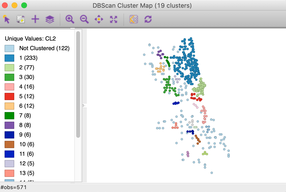
Figure 10: DBSCAN cluster map with d=3000 and MinPts = 4

In rare instances, a cluster may be identified that has less than the Min Points specified. This is an artifact of the treatment of Border points in the algorithm. Since border points are assigned to the first cluster to which they are connected, they are no longer available for inclusion in a later cluster. Say a later core point is connected to the same border point, which is counted as part of the Min Points for the new core. However, since it is already assigned to another cluster, it is no longer available and the new cluster seems to have fewer members than the specified Min Points. This particular feature of the DBSCAN algorithm can lead to counterintuitive results, although this rarely happens. We illustrate such an instance below.⁶

Sensitivity analysis

We further assess the sensitivity of the cluster results to the two main parameters by increasing Min Points to 10, while keeping the distance at 3000. The corresponding cluster map is shown in Figure 11. The number of clusters is drastically reduced to 6, ranging in size from 110 to 12. In all, 310 points (more than half) are designated as noise.

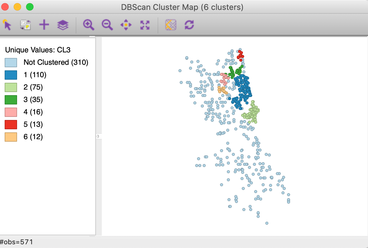
Figure 11: DBSCAN cluster map with d=3000 and MinPts = 10

Finally, we decrease the distance to 1000, while keeping Min Points at 4. In Figure 12, we now find 21 clusters, with the largest one consisting of 12 observations, whereas the smallest one has only 3 observations. A majority of the points (456) are not assigned to any cluster.

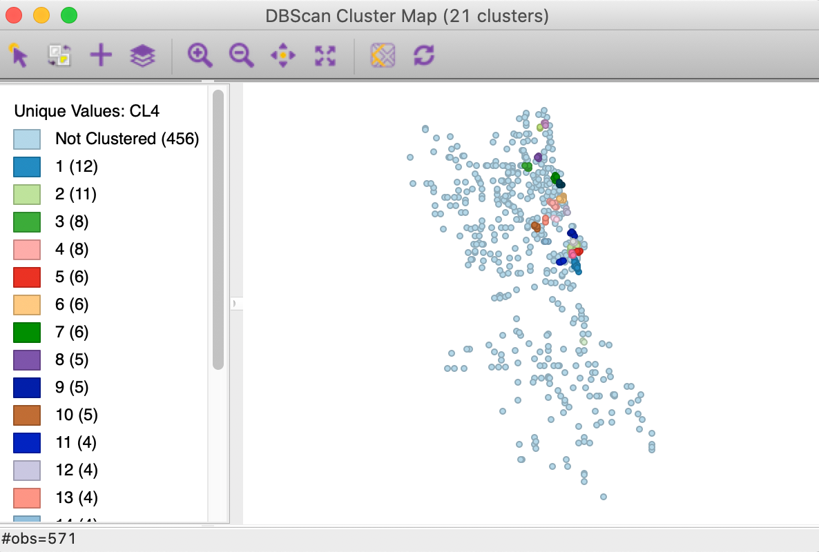
Figure 12: DBSCAN cluster map with d=1000 and MinPts = 4

Note that this is an instance where a cluster (cluster 21) has less than Min Points observations assigned to it. Consider the close up view in Figure 13, which gives the connectivity structure that corresponds to a distance band of 1000. Cluster 21 consists of points with id 501, 72 and 807. Point 501 is clearly a Core point, since it is connected to 72 and 807, as well as to 710, so it has three neighbors and meets the Min Points criterion of 4. Both 72 and 807 are assigned to 501 as Border points, since they do not meet the minimum connectivity requirement (each only has two neighbors). The same is the case for 710, but since 710 is already assigned to a different cluster (cluster 2), it cannot be reassigned to cluster 21. As a result, the latter only has 3 observations.

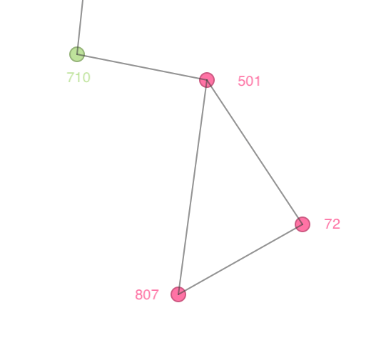
Figure 13: Border points in DBSCAN clusters

DBSCAN*

Principle

As we have seen, one of the potentially confusing aspects of DBSCAN is the inclusion of so-called Border points in a cluster. The DBSCAN* algorithm, outlined in Campello, Moulavi, and Sander (2013) and further elaborated upon in Campello et al. (2015), does away with the notion of border points, and only considers Core and Noise points.

Similar to the approach in DBSCAN, a Core object is defined with respect to a distance threshold (\(\epsilon\)) as the center of a neighborhood that contains at least Min Points other observations. All non-core objects are classified as Noise (i.e., they do not have any other point within the distance range \(\epsilon\)). Two observations are \(\epsilon\)-reachable if each is part of the \(\epsilon\)-neighborhood of the other. Core points are density-connected when they are part of a chain of \(\epsilon\)-reachable points. A cluster is then any largest (i.e., all eligible points are included) subset of density connected pairs. In other words, a cluster consists of a chain of pairs of points that belong to each others \(\epsilon\)-neighborhoods.

An alternative way to view \(\epsilon\)-reachability is to consider the minimum radius such that two points satisfy this criterion for a given Min Points, or k, where k = Min Points - 1 (more precisely, whereas Min Points includes the point itself, k does not). For k > 1 (or, Min Points > 2), this is the so-called mutual reachability distance, the maximum between the distance needed to include the required number of neighbors for each point (the k-nearest neighbor distance, called core distance in HDBSCAN, \(d_{core}\), see below) and the actual inter-point distance. This has the effect of pushing points apart that may be close together, but otherwise are in a region of low density, so that their respective k-nearest neighbor distances are (much) larger than the distance between them. Formally, the concept of mutual reachability distance between points A and B is defined as: \[d_{mr}(A,B) = max[d_{core}(A),d_{core}(B),d_{AB}].\] The mutual reachibility distance between the points forms the basis to construct a minimum spanning tree (MST) from which a hierarchy of clusters can be obtained. The hiearchy follows from applying cuts to the edges in the MST in decreasing order of core distance.

Conceptually, this means that one starts by applying a cut between two edges that are the furthest apart. This either results in a single point splitting off (a Noise point), or in the single cluster to split into two (two subtrees of the MST). Subsequent cuts are applied for smaller and smaller distances. Decreasing the critical distance is the same as increasing the density of points, referred to as \(\lambda\) (see below for a formal definition).

As Campello et al. (2015) show, applying cuts to the MST with decreasing distance (or increasing density) is equivalent to applying cuts to a dendrogram obtained from single linkage hierarchical clustering using the mutual reachability distance as the dissimilarity matrix.

DBSCAN* derives a set of flat clusters by applying a cut to the dendrogram associated with a given distance threshold. The main differences with the original DBSCAN is that border points are no longer considered and the clustering process is visualized by means of a dendrogram. However, in all other respects it is similar in spirit, and it still suffers from the need to select a distance threshold.

HDBSCAN (or HDBSCAN*) improves upon this by eliminating the arbitrariness of the threshold. This is considered next.

Implementation

DBSCAN* is invoked from the cluster menu as Clusters > DBSCAN in the same way as DBSCAN, but by selecting the Method as DBSCAN* . This also activates the Min Cluster Size option, set to equal to Min Points by default. The latter is initialized at 4. As shown in Figure 14, the starting point for the Distance Threshold is again the distance that ensures that each point has at least one neighbor. The value is in feet, which follows from using Raw for the Transformation, to keep the original coordinate units. Since this max-min value is typically not a very informative distance, we will change it to 3000. All the other settings are the same as before.

Figure 14: DBSCAN* parameters

After invoking Run, the dendrogram is populated, as shown in Figure 15. The horizontal scale shows the mutual reachability distance, and the cut line (dashed red line) is positioned at 3000. This yields 12 clusters, color coded in the graph. As was the case for classical hierarchical clustering, the dendrogram supports linking and brushing (not illustrated here).

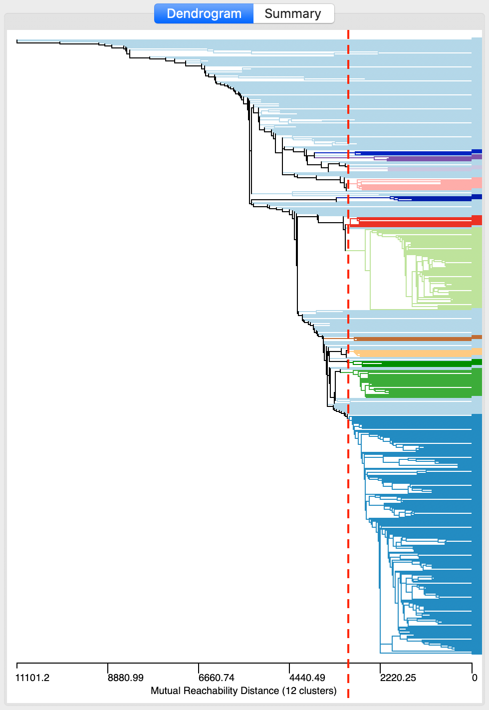
Figure 15: DBSCAN* dendrogram for d=3000 and MinPts=4

Save/Show Map saves the cluster classification to the data table and renders the corresponding cluster map, as in Figure 16. The 12 clusters range in size from 221 to 4, with 194 observations classified as noise. They follow the same general pattern as for DBSCAN in Figure 10, but seem more compact. Recall, the latter yielded 19 clusters ranging in size from 233 to 4, with 122 noise points.

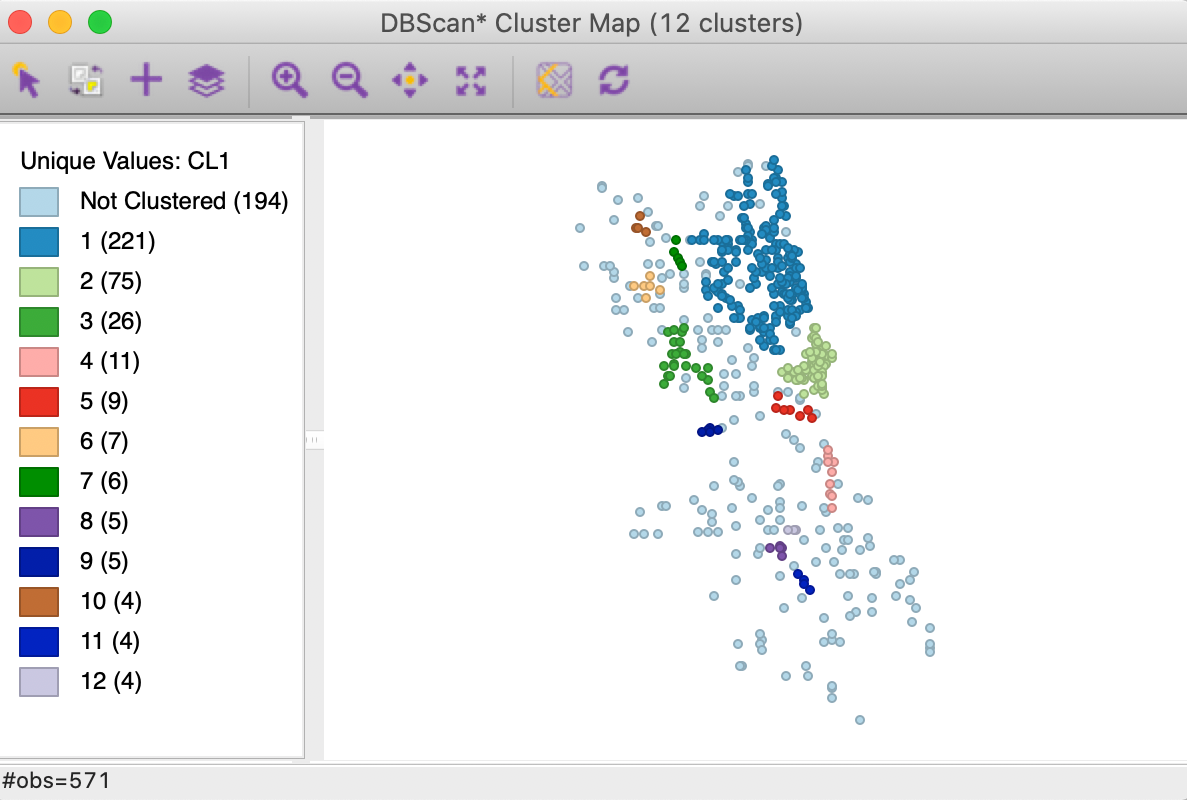
Figure 16: DBSCAN* cluster map with d=3000 and MinPts=4

In addition to the cluster map, the Summary panel contains the usual measures of fit, which are not that meaningful in this context.

Exploring the dendrogram

As long as Min Points (and the minimum cluster size) remains the same, we can explore the dendrogram for different threshold distance cut values. This can be accomplished by moving the cut line in the graph, or by typing a different value in the Distance Threshold box. For example, in Figure 17, the cut line has been moved to 2000. There are still 12 clusters, but their makeup is quite different from before.

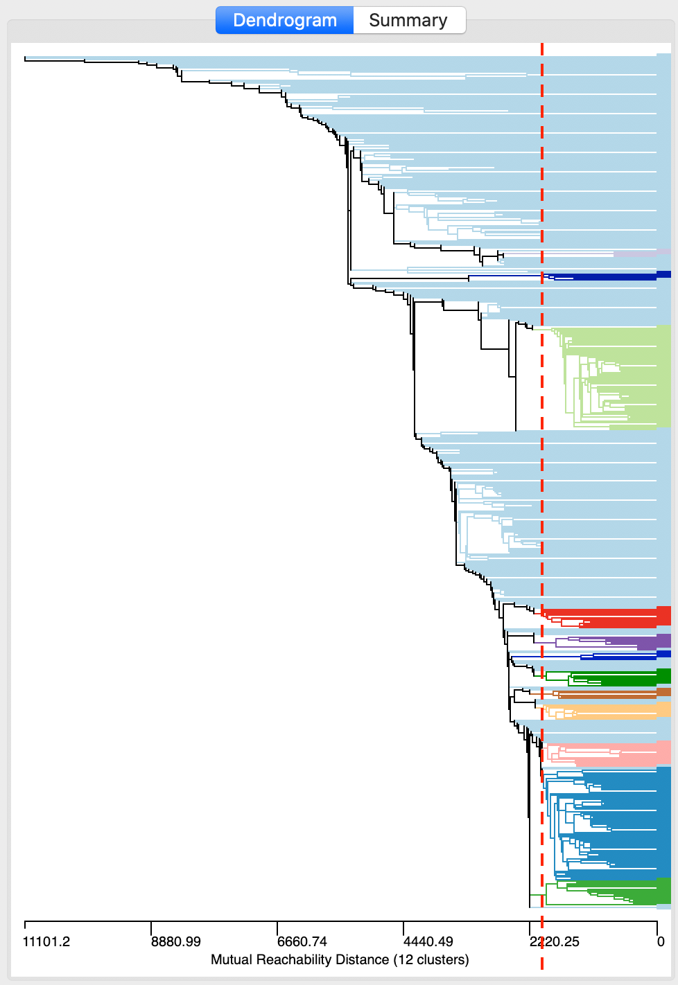
Figure 17: DBSCAN* dendrogram for d=2000 and MinPts=4

As we see in the cluster map in Figure 18, the clusters are now much smaller, ranging in size from 74 to 4, with 334 noise points. More interestingly, it seems like the large cluster in the northern part of the city (cluster 1 in Figure 16) is being decomposed into a number of smaller sub-clusters.

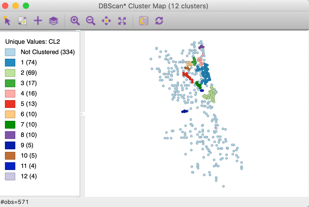
Figure 18: DBSCAN* cluster map with d=2000 and MinPts=4

Note that for a different value of Min Points, the dendrogram needs to be reconstructed, since this critically affects the mutual reachability distance (through the new core distance).

The main advantage of DBSCAN* over DBSCAN is a much more straightforward treatment of Border points (they are all classified as Noise), and an easy visualization of the sensitivity to the threshold distance by means of a dendrogram. However, just as for DBSCAN, the need to select a fixed threshold distance (to obtain a flat cluster) remains an important drawback.

HDBSCAN

Principle

HDBSCAN was originally proposed by Campello, Moulavi, and Sander (2013), and more recently elaborated upon by Campello et al. (2015) and McInnes and Healy (2017).⁷ As in DBSCAN*, the algorithm implements the notion of mutual reachability distance. However, rather than applying a fixed value of \(\epsilon\) or \(\lambda\) to produce a level set, a hierarchical process is implemented that finds an optimal set of clusters. This allows for different levels of \(\lambda\) for each cluster. In order to accomplish this, the concept of cluster stability or persistence is introduced. Optimal clusters are selected based on their relative excess of mass value, which is a measure of their persistence.

HDBSCAN keeps the notion of Min Points from DBSCAN, but introduces the concept of core distance of an object (\(d_{core}\)) as the distance between an object and its k-nearest neighbor, where k = Min Points - 1 (in other words, as for DBSCAN, the object itself is included in Min Points).

Intuitively, for the same k, the core distance will be much smaller for densely distributed points than for sparse distributions. Associated with the core distance for each object \(p\) is an estimate of density or \(\lambda_p\) as the inverse of the core distance. As the core distance becomes smaller, \(\lambda\) increases, indicating a higher density of points.

As in DBSCAN*, the mutual reachability distance is employed to construct a minimum spanning tree, or, rather, the associated dendrogram from single linkage clustering. In constrast to DBSCAN*, there is not a global cut applied to the dendrogram that uses the same value of \(\lambda\) for all clusters. Instead, HDBSCAN derives an optimal solution, based on the notion of persistence or stability of the cluster. A detailed illustration of these concepts and their implementation in the algorithm is given in the Appendix. Next, we consider each of these concepts more formally.

Persistence

As the value of \(\lambda\) increases (or, equivalently, the core distance becomes smaller), larger clusters break into subclusters (our analogy with rising ocean levels), or shed Noise points. Note that a Noise point dropping out is not considered a split of the cluster. The cluster remains, but just becomes smaller.

The objective is to identify the most prominent clusters as those that continue to exist longest. This is formalized through the concept of excess of mass (Müller and Sawitzki 1991), or the total density contained in a cluster after it is formed, i.e., after a level \(\lambda_{min}\) is reached.

In our island analogy, \(\lambda_{min}\) would correspond to the ocean level where the land bridge is first covered by water, such that the islands are no longer connected and appear as separate entities. The excess of mass would be the volume of the island above that ocean level, as illustrated in Figure 19. At the highest density (p in the Figure), two separate clusters are shown on the left, which appear at p = 0.10. With lower density, they are united into a single cluster, which appears around 0.03. At that level, there is an additional smaller cluster as well. With density below this level, there are no separate clusters.

Figure 19: Excess of mass (Source: Stuetzle and Nugent 2010)

More formally, a notion of relative excess of mass of a cluster \(C_i\) that appears at level \(\lambda_{min}(C_i)\) is used to define the stability or persistence of a cluster \(C_i\) as: \[S(C_i) = \sum_{x_j \in C_i} (\lambda_{max}(x_j,C_i) - \lambda_{min} C_i),\] where \(\lambda_{min} C_i\) is the minimum density level at which \(C_i\) exists, and \(\lambda_{max}(x_j,C_i)\) is the density level after which point \(x_j\) no longer belongs to the cluster.

In Figure 19, we see how the cluster on the left side comes into being at p = 0.03. At p = 0.10, it splits into two new clusters. So, for the large cluster, \(\lambda_{min}\), or the point where the cluster comes into being is 0.03. The cluster stops existing (it splits) for \(\lambda_{max}\) = 0.10. In turn, p = 0.10 represents \(\lambda_{min}\) for the two smaller clusters.

A condensed dendrogram is obtained by evaluating the stability of each cluster relative to the clusters into which it splits. If the sum of the stability of the two descendants is larger than the stability of the parent node, then the two children are kept as clusters and the parent is discarded. Alternatively, if the stability of the parent is larger than that of the children, the children and all their descendants are discarded. In other words, the large cluster is kept and all the smaller clusters that descend from it are eliminated. Here again, a split that sheds a single point is not considered a cluster split, but only a shrinking of the original cluster (which retains its label). Only true splits that result in subclusters that contain at least two observations are considered in the simplification of the tree. Sometimes a further constraint is imposed on the minimum size of a cluster, which would pertain to the splits as well. As suggested in Campello et al. (2015), a simple solution is to set the minimum cluster size equal to Min Points.

For example, in the illustration in Figure 19, the area in the left cluster between 0.03 and 0.10 is larger than the sum of the areas in the smaller clusters obtained at 0.10. As a result, the latter would not be considered as separate clusters.

This yields a much simpler tree and an identification of clusters that maximize the sum of the individual cluster stabilities.

The C++ software implementation of HDBSCAN in GeoDa is based on the Python code published in McInnes, Healy, and Astels (2017).

Cluster membership

The first distance for which a point can become part of a cluster is \(d_{p,core}\), i.e., the k-nearest neighbor distance that satisfies the Min Points criterion. The inverse of this distance is an estimate of density associated with that entry point, or \(\lambda_p = 1 / d_{p,core}\). Once a point is part of a cluster, it remains there until the threshold distance becomes small enough such that all the points in the cluster become Noise. This smallest distance, \(d_{min}\), corresponds with the largest density, or, \(\lambda_{max} = 1/d_{min}\). The strength of the cluster membership of point \(p\) can now be expressed as the ratio of the smallest core distance for the cluster to the core distance for point p, \(d_{min} / d_{p,core}\), or, equivalently, as the ratio of the density that corresponds to the point’s core distance to the maximum density, or, \(\lambda_p / \lambda_{max}\).

This ratio gives a measure of the degree to which a point belongs to a cluster. For example, for points that meet the \(d_{min}\) thresholds, i.e., observations in the highest density region, the ratio will be 1. On the other hand, for Noise points, the ratio is set to 0. Points that are part of the cluster, but do not meet the strictest density criterion will have a value smaller than 1. The higher the ratio, the stronger the membership of the point in the corresponding cluster.

This ratio can be exploited as the basis of a soft or fuzzy clustering approach, in which the degree of membership in a cluster is considered. This is beyond our scope. Nevertheless, the ratio, or probability of cluster membership, remains a useful indicator of the extent to which the cluster is concentrated in high density points.

Outlier detection

An interest related to the identification of density clusters is to find points that do not belong to a cluster and are therefore classified as outliers. Parametric approaches are typically based on some function of the spread of the underlying distribution, such as the well-known 3-sigma rule for a normal density.⁸

An alternative approach is based on non-parametric principles. Specifically, the distance of an observation to the nearest cluster can be considered as a criterion to classify outliers. We already saw a form of this with the Noise points in DBSCAN, i.e., points that are too far from other points (given a neighborhood radius, or Eps) to be considered members of a cluster.

Campello et al. (2015) proposed a post-processing of the HDBSCAN results to characterize the degree to which an observation can be considered an outlier. The method is referred to as GLOSH, which stands for Global-Local Outlier Scores from Hierarchies.

The logic underlying the outlier detection is closely related to the notion of cluster membership just discussed. In fact, the probability of being an outlier can be seen to be the complement of the cluster membership.

The rationale behind the index is to compare the lowest density threshold for which the point is attached to a cluster (\(\lambda_p\) in the previous discussion) and the highest density threshold \(\lambda_{max}\). The GLOSH index for a point \(p\) is then: \[\mbox{GLOSH}_p = \frac{\lambda_{max} - \lambda_p}{\lambda_{max}},\] or, equivalently, \(1 - \lambda_p / \lambda_{max}\), the complement of the cluster membership for all but Noise points. For the latter, since the cluster membership was set to zero, the actual \(\lambda_{max}\) needs to be used. Given the inverse relationship between density and distance threshold, an alternative formulation of the outlier index is as: \[\mbox{GLOSH}_p = 1 - \frac{d_{min}}{d_{p,core}}.\]

Implementation

HDBSCAN is invoked from the Menu or the cluster toolbar icon as the second item in the density clusters subgroup, Clusters > HDBSCAN, as in Figure 20.

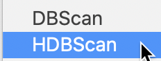
Figure 20: HDBSCAN option

The overall setup is very similar to that for DBSCAN, except that there is no threshold distance. The two main parameters are Min Cluster Size and Min Points. These are typically set to the same value, but there may be instances where a larger value for Min Cluster Size is desired. The Min Points parameter drives the computation of the core distance for each point, which forms the basis for the construction of the minimum spanning tree. As before, we make sure that the Transformation is set to Raw, as in Figure 21.

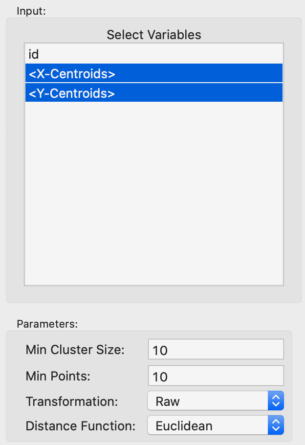
Figure 21: HDBSCAN input parameters

The first item that appears after selecting Run is the dendrogram representation of the minimum spanning tree, shown in Figure 22. This is mostly for the sake of completeness, and to allow for comparisons with HDBSCAN*. In and of itself, the raw dendrogram is not of that much interest. One interesting feature of the dendrogram is that it supports linking and brushing, which makes it possible to explore what branches in the tree subsets of points or clusters belong to (selected in one of the maps). The reverse is supported as well, so that branches in the tree can be selected and their counterparts identified in other maps and graphs.

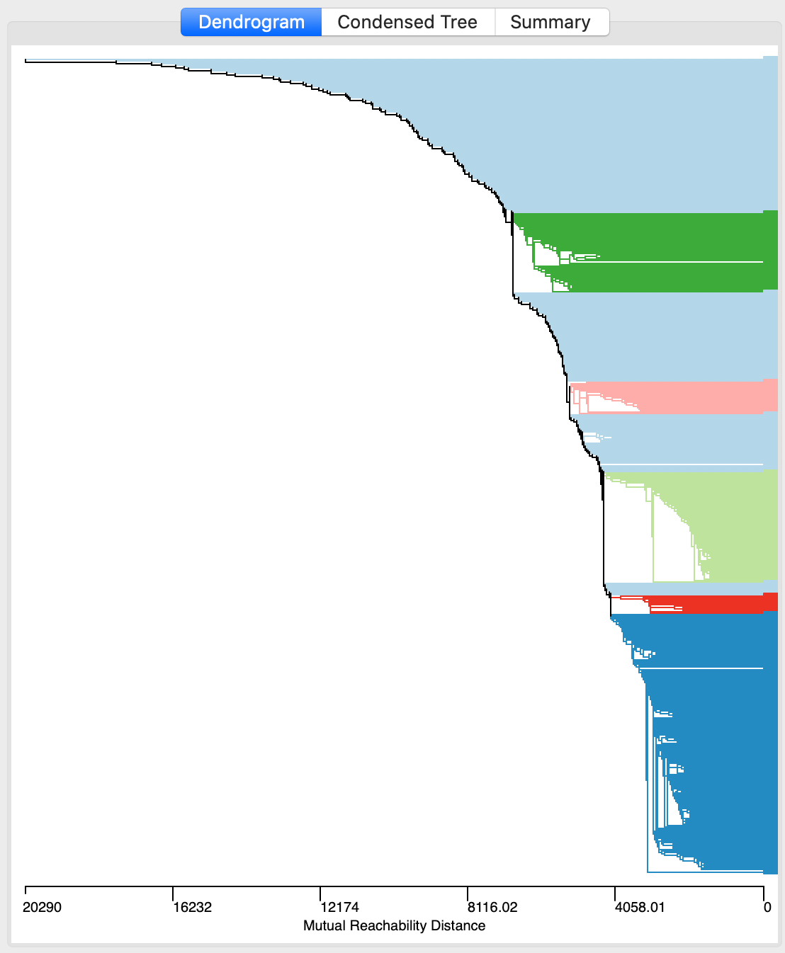
Figure 22: HDBSCAN dendrogram, Min Points = 10

In addition to the dendrogram, a cluster map is generated, with the cluster categories saved to the data table. In our example, as seen in Figure 23, there are five clusters, ranging in size from 181 to 13 observations. There are 221 noise points. The overall pattern is quite distinct from the results of DBSCAN and DBSCAN*, showing more clustering in the southern part of the city. For example, compare to the cluster map for DBSCAN with d = 3000 and MinPts = 10, shown in Figure 11, where the six clusters are all located in the nothern part of the city.

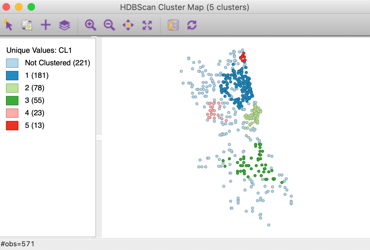
Figure 23: HDBSCAN cluster map, Min Points = 10

As for the other clustering methods, the usual measures of fit are contained in the Summary panel.

Exploring the condensed tree

An important and distinct feature of the HDBSCAN method is the visualization of cluster persistence (or stability) in the condensed tree or condensed dendrogram. This is invoked by means of the middle button in the results panel. The tree visualizes the relative excess of mass that results in the identification of clusters for different values of \(\lambda\). Starting at the root (top), with \(\lambda\) = 0, the left hand axis shows how increasing values of \(\lambda\) (going down) results in branching of the tree. Note how the shaded areas are not rectangles, but they gradually taper off, as single points are shedded from the main cluster.

The optimal clusters are identified by an oval with the same color as the cluster label in the cluster map. The shading of the tree branches corresponds to the number of points contained in the branch, with lighter suggesting more points.

In our application, the corresponding tree is shown in Figure 24. We see how some clusters correspond with leaf nodes, whereas others occur at higher stages in the tree. For example, cluster 1, the left-most cluster in the tree takes precedence over its descendants. In contrast, the second cluster from left (cluster 5) is the last node of the branch, which exists until all its elements become singletons (or, are smaller than the minimum cluster size).

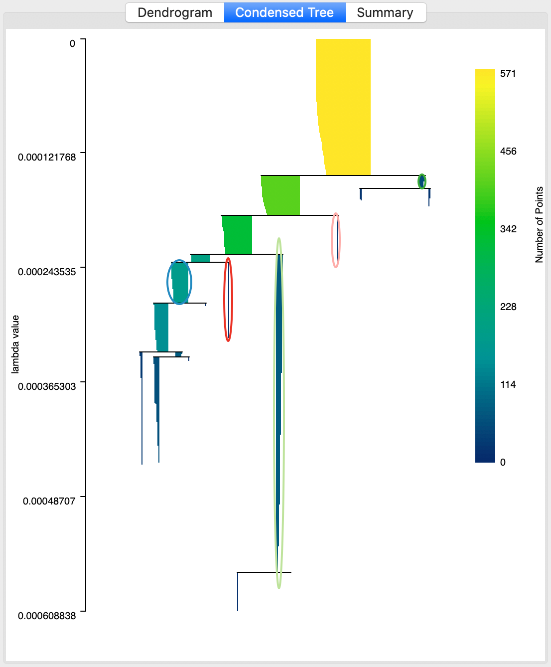
Figure 24: HDBSCAN condensed dendrogram, Min Points = 10

The condensed tree supports linking and brushing as well as a limited form of zoom operations. The latter may be necessary for larger data sets, where the detail is difficult to distinguish in the overall tree. Zooming is implemented as a specialized mouse scrolling operation, slightly different in each system. For example, on a MacBook track pad, this works by moving two fingers up or down. There is no panning, but the focus of the zoom can be moved to specific subsets of the graph.

Figure 25 illustrates this feature. All points belonging to cluster 1 are selected in the cluster map, and the corresponding observations are highlighted in red in the zoomed in condensed tree. While some observations are shedded in the core part of the cluster (the area surrounded by the oval), we see how many only disappear from the cluster at lower nodes in the tree. However, the relative excess of mass of those lower branches was dominated by the one of the parent node, hence its selection as the cluster.

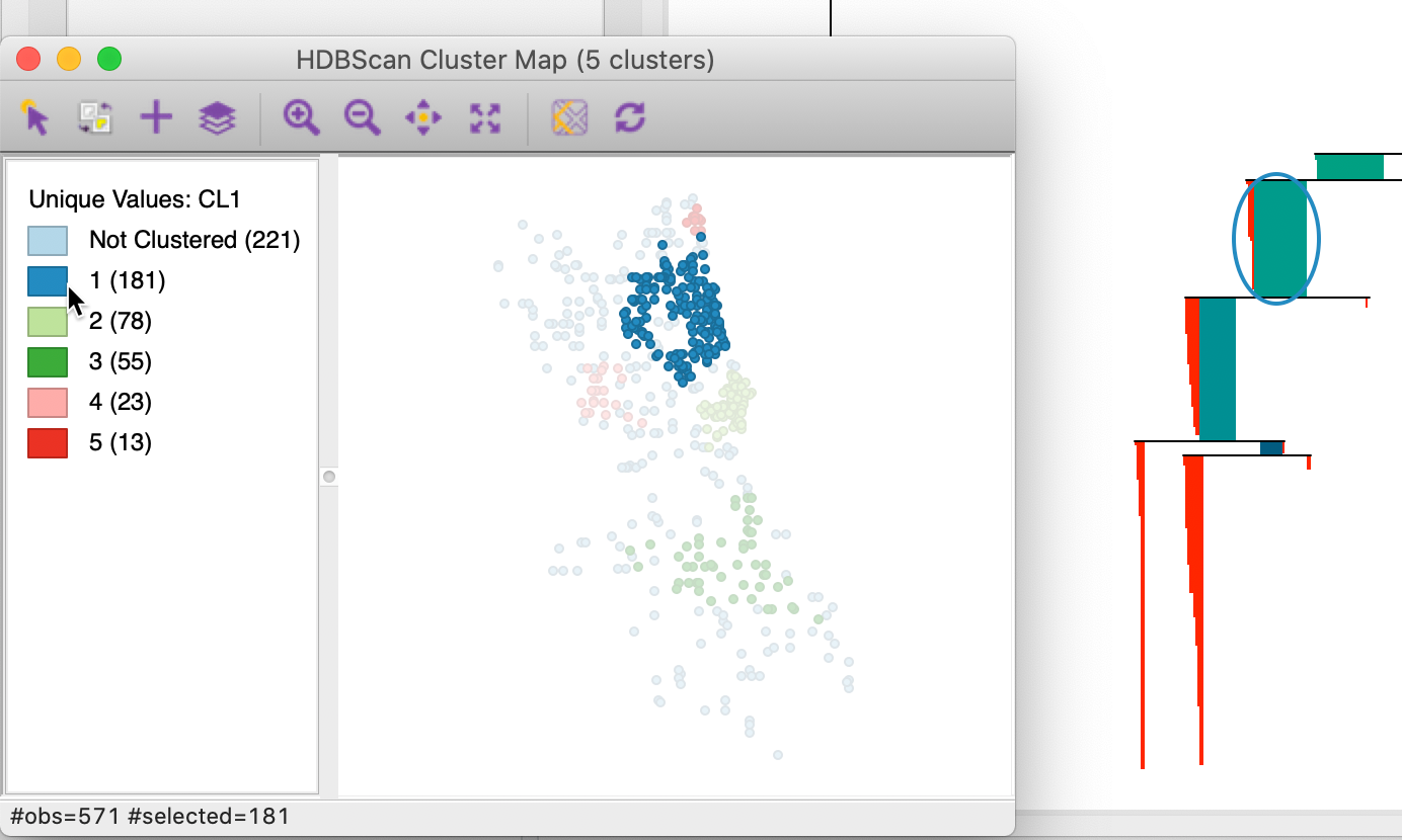
Figure 25: HDBSCAN zooming in on the condensed dendrogram, Min Points = 10

Cluster membership

The Save button provides the option to add the core distance, cluster membership probability and outlier index (GLOSH) to the data table. The interface, shown in Figure 26, suggests default names for the variables, but in most instances one will want to customize those.

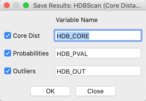
Figure 26: HDBSCAN save results option

The membership probability provides some useful insight into the strength of the clusters. For example, in Figure 27, the 23 observations that belong to cluster 4 have been selected in the data table (and moved to the top). The column labeled HDB_PVAL lists the probabilities. The column labeled HDB_CORE shows the core distance for each point. Clearly, points are grouped in the same cluster with a range of different core distances, corresponding to different values of \(\lambda\).

Ten of the 23 points have a probability of 1.0, which means that they meet the strictest \(\lambda\) criterion for the cluster. The other values range from 0.961 to 0.786, suggesting a quite strong degree of overall clustering.

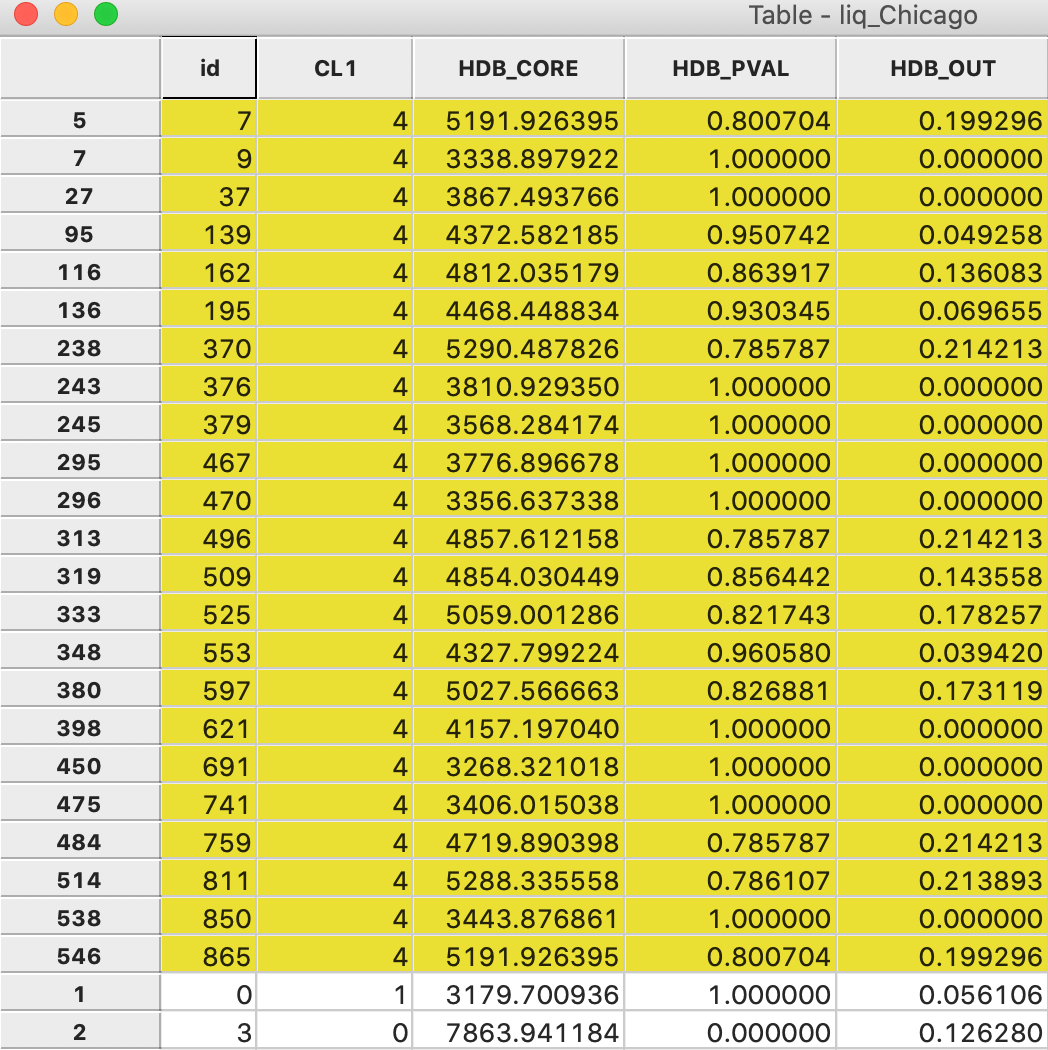
Figure 27: HDBSCAN cluster 4 membership strength

The probabilities can be visualized in any map in order to further visualize the strength of cluster membership for a particular cluster. For example, in Figure 28, the points in cluster 4 are selected in the cluster map on the left, and their probability values are visualized in a natural breaks map on the right. This clearly illustrates how points further from the core of the cluster have lower probabilities.

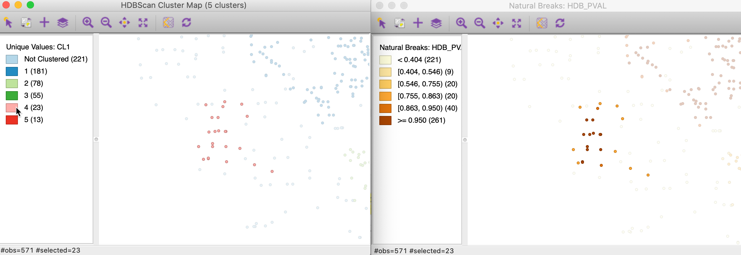
Figure 28: HDBSCAN cluster 4 membership strength map

Outliers

A final characteristic of the HDBSCAN output is the GLOSH outlier index, contained in the data table as the column HDB_OUT. In Figure 29, this column has been sorted in descending order, showing the points with id 185 and 630 with an outlier index of respectively 0.661 and 0.614. These observations correspond to two points in the very southern part of the city and they appear quite separated from the nearest cluster (cluster 3, the southernmost cluster). The two points are surrounded by other Noise points and are far removed from cluster 3.

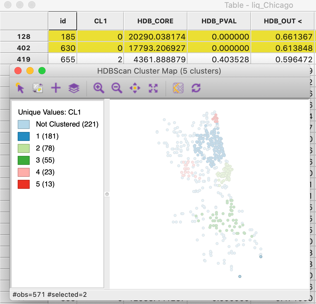
Figure 29: HDBSCAN outliers

As any other variable in the data table, the outlier index can be mapped to provide further visual interpretation of these data patterns.

Appendix

DBSCAN worked example

In order to illustrate the logic behind the DBSCAN algorithm, we consider a toy example of 9 points, the coordinates of which are listed in Figure 30.

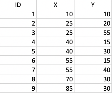
Figure 30: Toy point data set

We can use GeoDa to create this as a point layer and use the distance weights functionality to obtain the connectivity structure that ensures that each point has at least one neighbor. From the weights characteristics, we find that for a distance of 29.1548, the number of neighbors ranges from 1 to 5. The matching connectivity graph is shown in Figure 31.

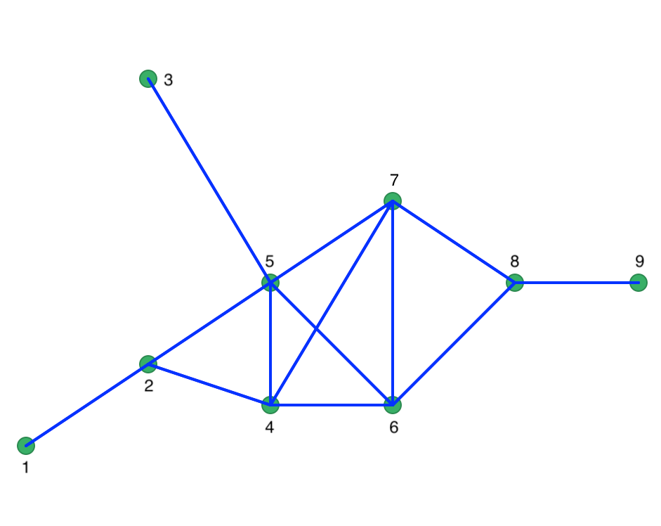
Figure 31: Connectivity graph for full connectivity

To illustrate the concept of Noise points (i.e., unconnected points for a given critical distance), we lower the distance cut-off to 20. Now, we have one isolate (point 3) and the maximum number of neighbors drops to 3. The corresponding connectivity graph is shown in Figure 32 with the matching weights in Figure 33.

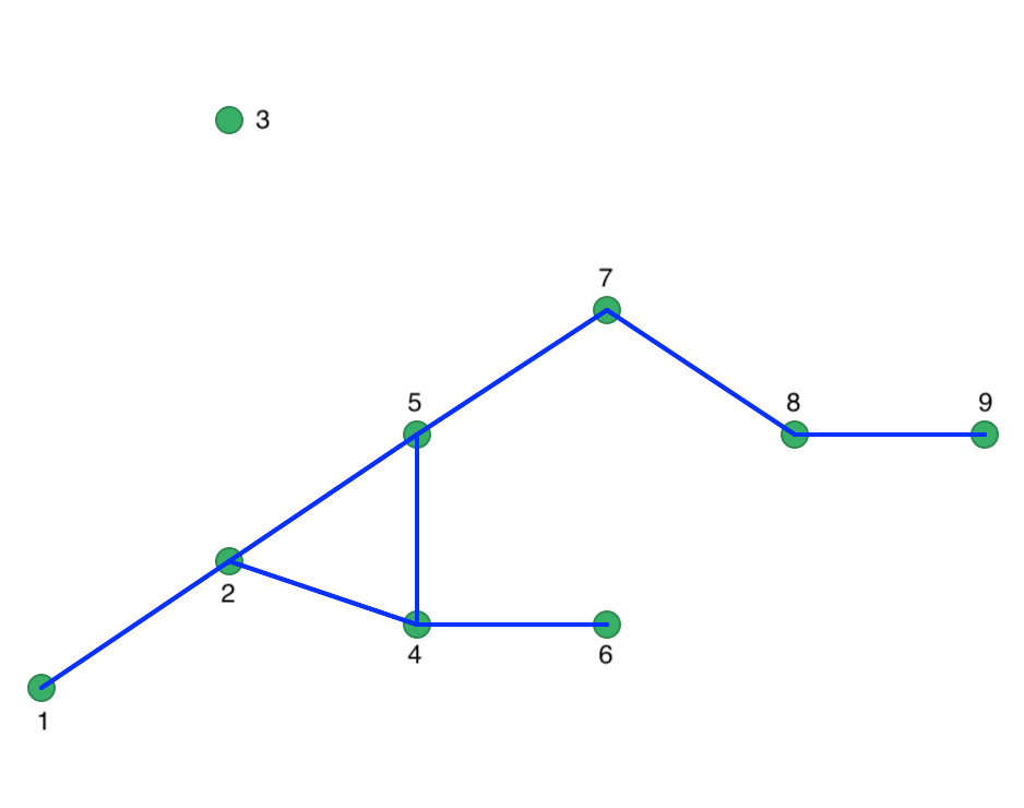
Figure 32: Connectivity graph for Eps = 20

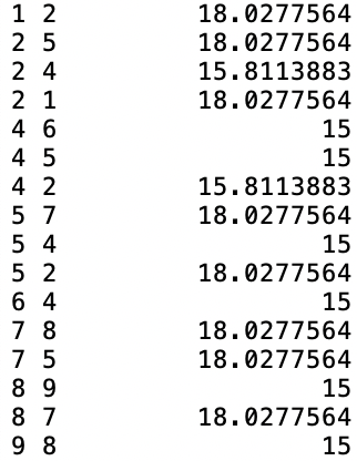
Figure 33: Spatial Distance Weights for Eps = 20

With MinPts as 4 (i.e., 3 neighbors for a core point), we can now move through each point, one at a time. Starting with point 1, we find that it only has one neighbor (point 2) and thus does not meet the MinPts criterion. Therefore, we label it as Noise for now. Next, we move to point 2. It has 3 neighbors, meaning that it meets the Core criterion and it is labeled cluster 1. All its neighbors, i.e., 1, 4 and 5 are also labeled cluster 1 and are no longer considered. Note that this changes the status of point 1 from Noise to Border. We next move to point 3, which has no neighbors and is therefore labeled Noise.

We move to point 6, which is a neighbor of point 4, which belongs to cluster 1. Since 6 is therefore density connected, it is added to cluster 1 (as a Border point). The same holds for point 7, which is similarly added to cluster 1.

Point 8 has two neighbors, which is insufficient to reach the MinPts criterion. Therefore, it is labeled Noise, since point 7 is not a Core point. Finally, point 9 has only point 8 as neighbor and is therefore also labeled Noise.

In the end, we have one cluster consisting of 6 points, shown as the dark blue points in Figure 34. The remaining points are Noise, labeled as light blue in the Figure. They are not part of any cluster.

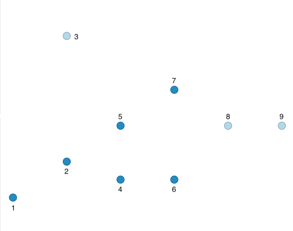
Figure 34: DBSCAN clusters for Eps = 20 and MinPts = 4

We illustrate a more interesting outcome by lowering Eps to 15 with MinPts at 2. As a result, the points are less connected, shown in the connectivity graph in Figure 35.

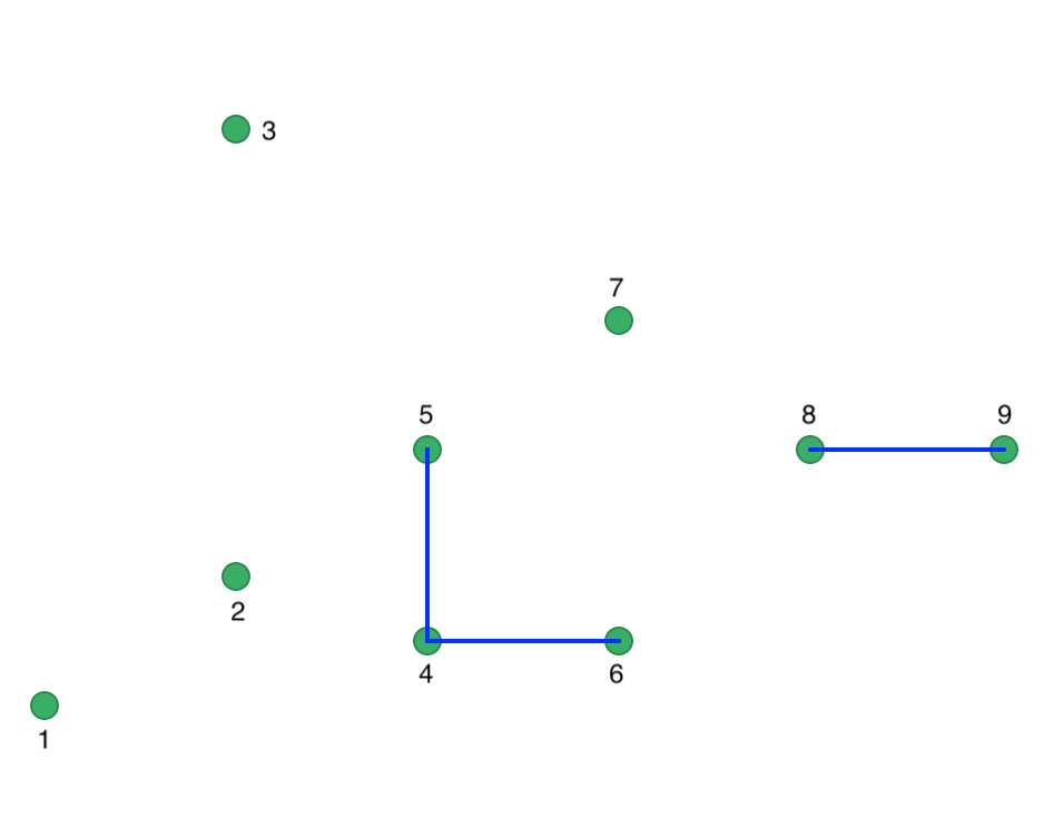
Figure 35: Connectivity graph for Eps = 15

Using the same logic as before, we find points 1, 2, and 3 to be unconnected. Point 4 is connected to 5 and 6, which meets the MinPts criterion and results in all three points being labeled cluster 1. Point 7 is again Noise, but points 8 and 9 are connected to each other, yielding cluster 2. The outcome is summarized in Figure 36, which shows four Noise points, a cluster consisting of 4, 5, and 6, and a cluster consisting of points 8 and 9.

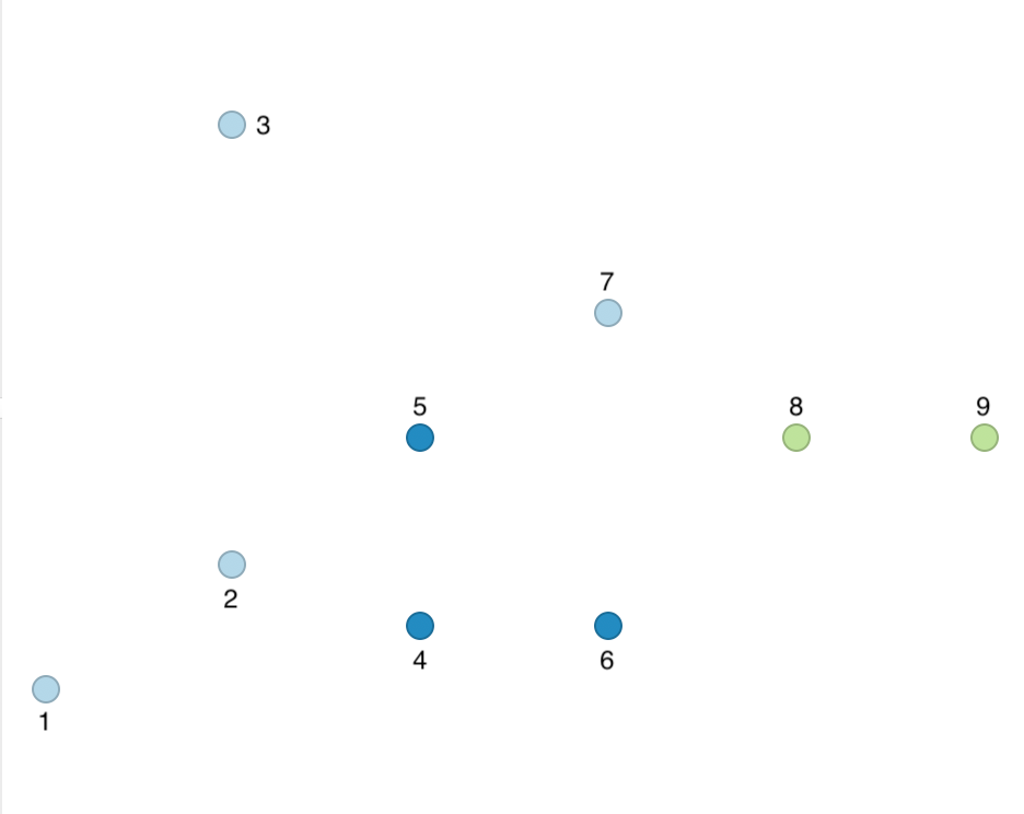
Figure 36: DBSCAN clusters for Eps = 15 and MinPts = 2

This example illustrates the sensitivity of the results to the parameters Eps and MinPts.

HDBSCAN worked example

We apply the HDBSCAN algorithm to the same nine points from Figure 30. We set Min Cluster Size and Min Points to 2. As a result, the mutual reachability distance is the same as the original distance, given in Figure 37. Since the core distance for each point is its nearest neighbor distance (smallest distance to have one neighbor), the maximum of the two core distances and the actual distance will always be the actual distance. While this avoids one of the innovations of the algorithm, it keeps our illustration simple.

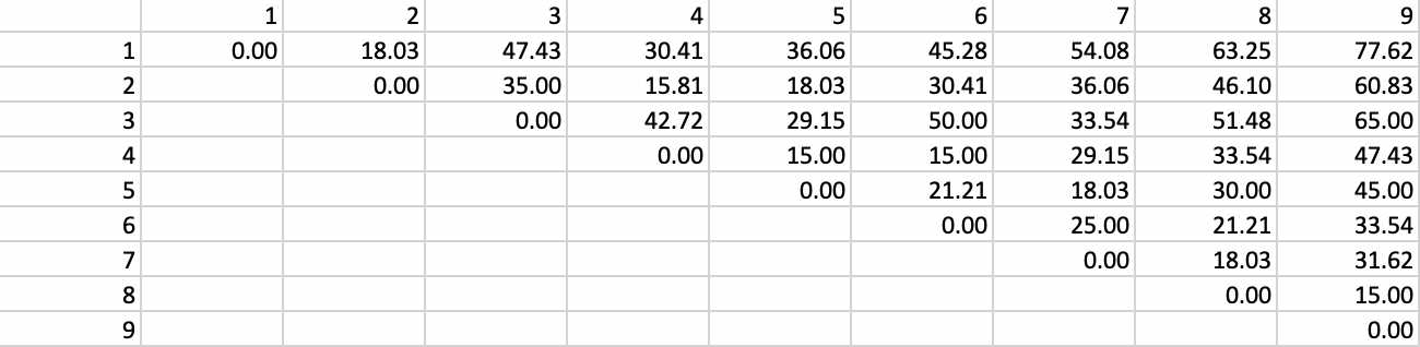
Figure 37: Distance matrix

The distance matrix can be used to find the core distance for each point as its nearest neighbor distance (the smallest element in a row of the distance matrix), as well as the associated \(\lambda_p\) value. The latter is simply the inverse of the core distance. These results are shown in Figure 38.

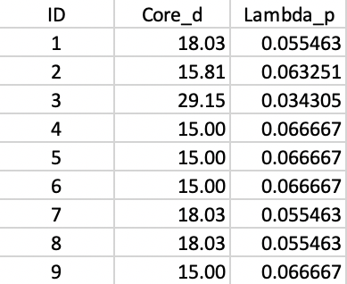
Figure 38: Core distance and lambda for each point

The distance matrix also forms the basis for a minimum spanning tree (MST), which is essential for the hierarchical nature of the algorithm. The MST is shown in Figure 39, with both the node identifiers and the edge weights listed (the distance between the two nodes the edge connects).

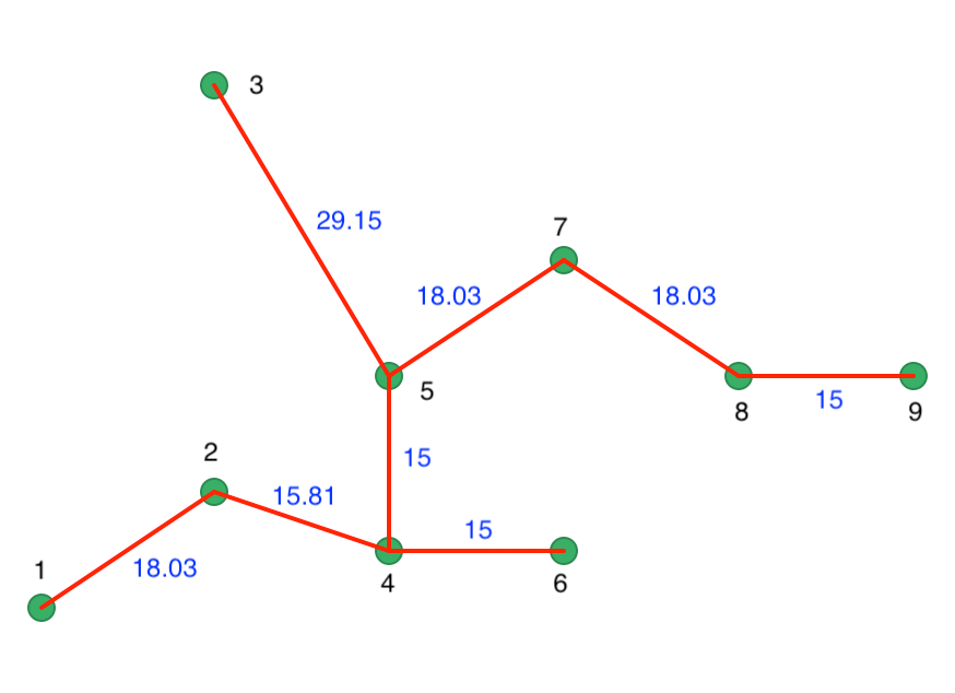
Figure 39: Minimum Spanning Tree

One interpretation of the HDBSCAN algorithm is to view it as a succession of cuts in the MST. These cuts start with the highest edge weight and move through all the edges in decreasing order of the weight. The first cut is illustrated in Figure 40, where 3 is separated from 5 as a result of its edge weight of 29.15.

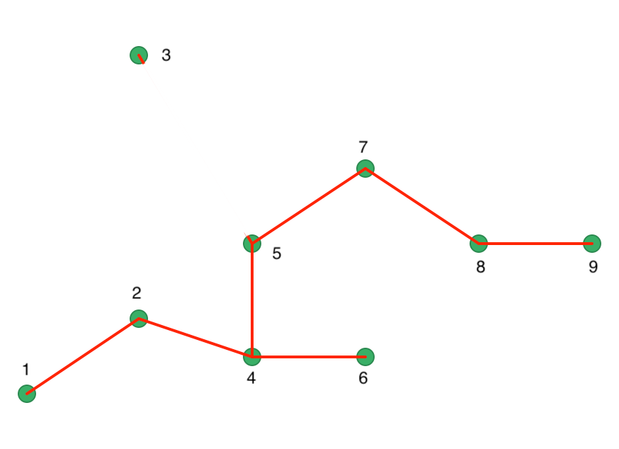
Figure 40: Minimum Spanning Tree - first cut

The next cut is a bit more problematic in our example, since both 1-2, 5-7, and 7-8 are separated by the same distance of 18.03. This is an artifact of our simple example, and is much less likely to occur in practice. We proceed with a cut 7 and 8, as shown in Figure 41. A different cut will yield a different solution for this example. We ignore that aspect in our illustration.

The process of selecting cuts continues until all the points are singletons and constitute their own cluster. Formally, this is equivalent to carrying out single linkage hierarchical clustering based on the mutual reachability distance matrix.

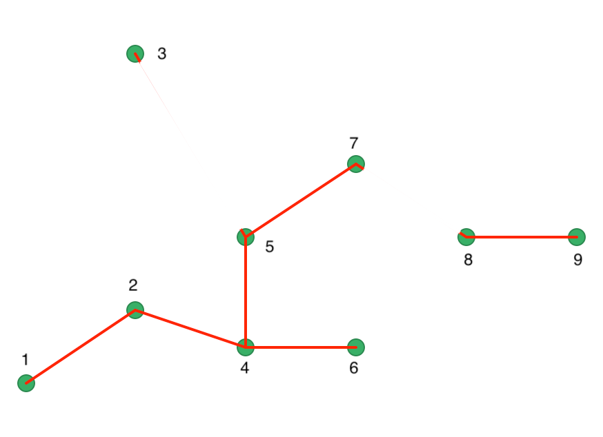
Figure 41: Minimum Spanning Tree - second cut

An alternative visualization of the pruning process is in the form of a tree, shown in Figure 42. In the root node, all the points form a single cluster. The corresponding \(\lambda\) level is set to zero. As \(\lambda\) increases, or, equivalently, the core distance decreases, points fall out of the cluster, or the cluster splits into two subclusters. This process continues until each point is a leaf in the tree (i.e., it is by itself).

We can think of this process using our island analogy. At first all points constitute a large island. As the ocean level rises, i.e., \(\lambda\) increases, points on the island become submerged, dropping out of the cluster. Alternatively, two hills on the island connected by a valley become separate as the ocean submerges the valley.

This process is formally represented in the tree in Figure 42. As \(\lambda\) reaches 0.034 (for a distance of 29.15), point 3 gets removed and becomes a leaf (in our island analogy, it becomes submerged). In the GeoDa implementation of HDBSCAN, singletons are not considered to be valid clusters, so we move on to node C1, which becomes the new root, with \(\lambda\) reset to zero.

The next meaningful cut is for \(\lambda = 0.055\), or a distance of 18.03. As we see from Figure 41, this creates two clusters, one consisting of the six points 1-7, but without 3, say C2, and the other consisting of 8 and 9, C3. The process continues for increasing values of \(\lambda\), although in each case the split involves a singleton and no further valid clusters are obtained. We consider this more closely when we examine the stability of the clusters.

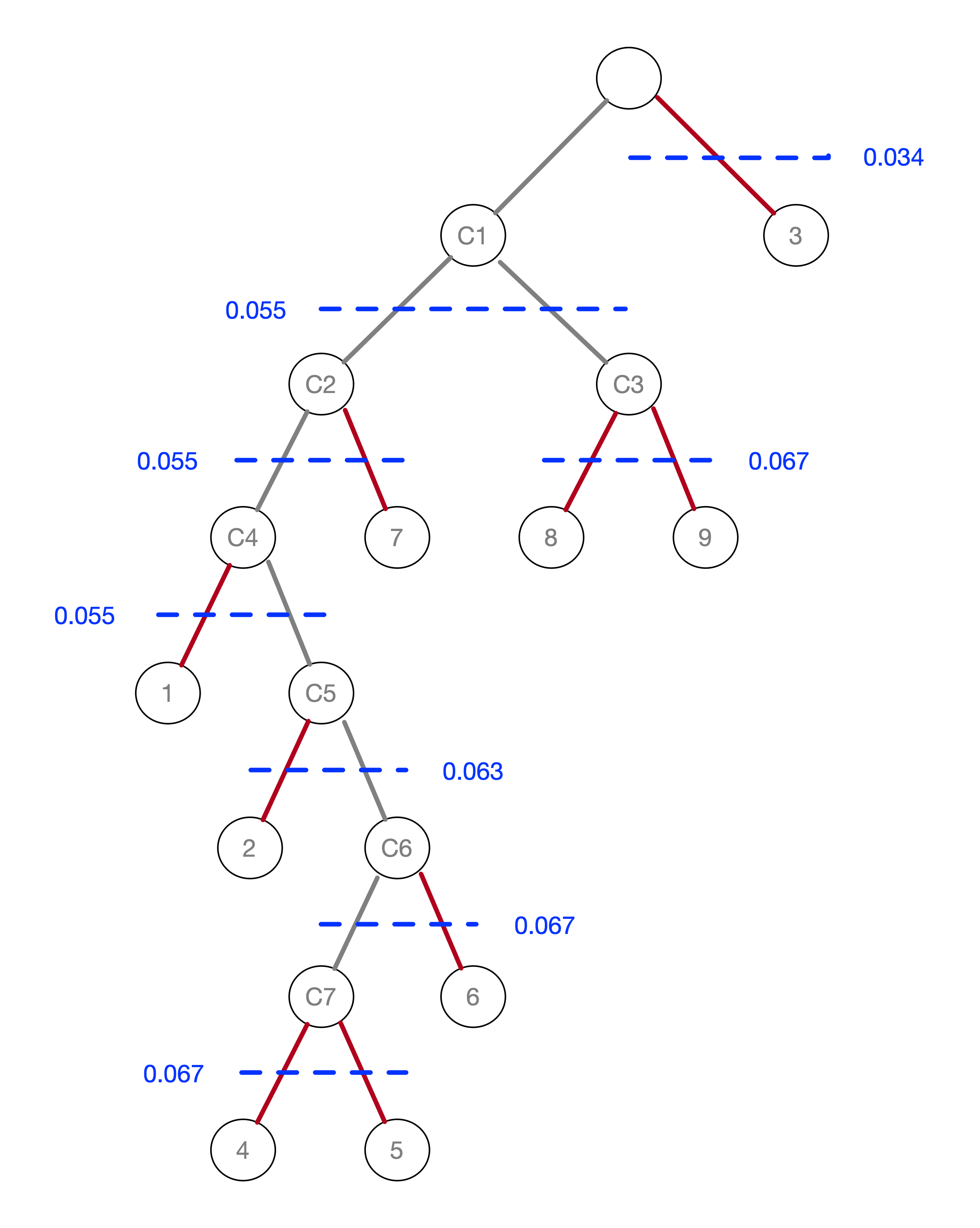
Figure 42: Pruning the MST

First, note how the \(\lambda_p\) values in Figure 38 correspond to the \(\lambda\) value where the corresponding point falls out of the clusters in the tree in Figure 42. For example, for point 7, this happens for \(\lambda\) = 0.055, or a core distance of 18.03. The stability or persistence of each cluster is defined as the sum over all the points of the difference between \(\lambda_p\) and \(\lambda_{min}\), where \(\lambda_{min}\) is the \(\lambda\) level where the cluster forms.

To make this concrete, consider cluster C3, which is formed (i.e., splits off from C1) for \(\lambda\) = 0.055463. Therefore, the value of \(\lambda_{min}\) for C3 is 0.055463. The value of \(\lambda_p\) for points 8 and 9 is 0.066667, corresponding with a distance of 15.0 at which they become singletons (or leaves in the tree). The contribution of each point to the persistence of the cluster C3 is thus 0.066667 - 0.055463 = 0.011204, as shown in Figure 43. The total value of the persistence of cluster C3 is therefore 0.022408. Similar calculations yield the persistence of cluster C2 as 0.041400. For the sake of completeness, we also include the results for cluster C1, although those are ignored by the algorithm, since C1 is reset as root of the tree.

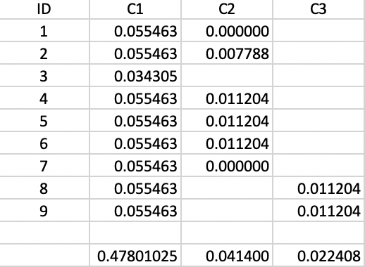
Figure 43: Cluster stability

The condensed tree only includes C1 (as root), C2 and C3. Since the persistence of a singleton is zero, and C4 includes one less point than C2, but with the same value for \(\lambda_{min}\), the sum of the persistence of C4 and 7 is less than the value for C2, hence the condensed tree stops there. This allows for two different values of \(\lambda\) to play a role in the clustering mechanism, rather than the single value that needs to be set a priori in DBSCAN.

To compare, consider the clusters that would result from setting \(\lambda\) = 0.055, or a core distance of 18.03, using the logic of DBSCAN* (no border points). From Figure 39, we see that this would result in a grouping of 8-9 and 2-4-5-6, with 1, 3 and 7 as noise points. In our tree, that would be represented by C3 and C5. The main contribution of HDBScan is that the optimal level of \(\lambda\) is determined by the algorithm itself, and is adjusted in function of the structure of the data, rather than having a one size fits all that needs to be specified beforehand.

The corresponding cluster map for our toy example is shown in Figure 44.

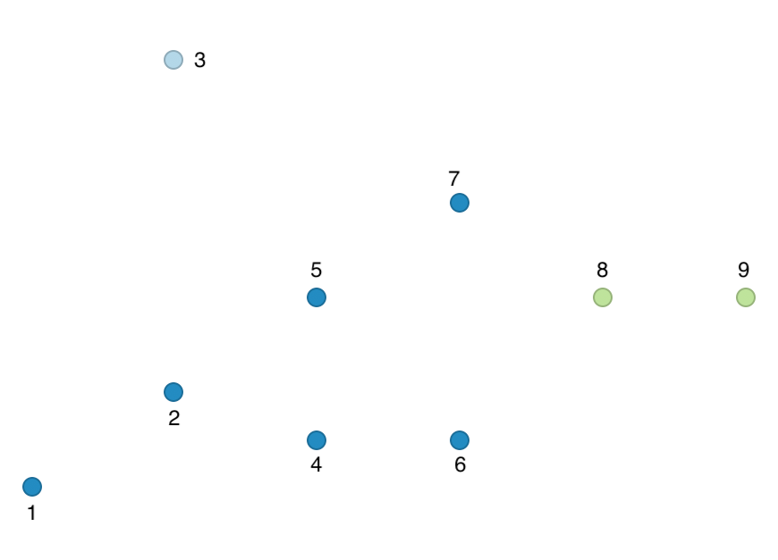
Figure 44: HDBScan cluster map - toy example

A final set of outputs from the algorithm pertains to soft clustering and the identification of outliers. GeoDa saves these values for each point, together with the associated core distance, as shown in Figure 45. The core distance is the same as in Figure 38. The probability or strength for each point to be part of a cluster is computed as the ratio of \(\lambda_p\) to \(\lambda_{max}\), with \(\lambda_{max}\) as the largest value of the individual \(\lambda_p\). Equivalently, this is the ratio of the smallest core distance over the core distance of point p. This is listed as HDB_PVAL in the table. For example, since \(\lambda_{max}\) is 0.066667 in our example, points 4-5-6 and 8-9 obtain a probability of 1.0, or certainty to be part of the cluster. In contrast, points 1, 2 and 7 have a lower value. For example, for point 7 the ratio is 15.0/18.03 = 0.832. For noise points, the probability is set to zero.

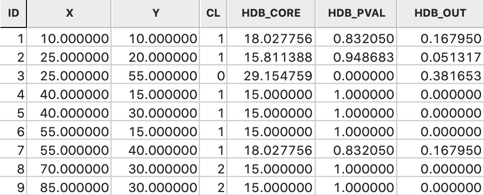
Figure 45: HDBScan saved results

The last piece of information is the probability that a point is an outlier. This is computed as \(1 - \lambda_p / \lambda_{max}\). For all but the noise points, this is the complement of the cluster probability. For example, for point 1, this is 1.0 - 0.0555/0.0667 = 1.0 - 0.832 = 0.168. However, for point 3, the noise point, the computation is slightly different. At first sight, one would expect the outlier probability to be 1.0. However, the \(\lambda_{max}\) for this point is the \(\lambda\) value for C1, or 0.055. Consequently the outlier probability is 1.0 - 0.034/0.055 = 0.382.

References

Campello, Ricardo J. G. B., Davoud Moulavi, and Jörg Sander. 2013. “Density-Based Clustering Based on Hierarchical Density Estimates.” In Advances in Knowledge Discovery and Data Mining. PAKDD 2013. Lecture Notes in Computer Science, Vol. 7819, edited by Jian Pei, Vincent S. Tseng, Longbing Cao, Hiroshi Motoda, and Guandong Xu, 160–72.

Campello, Ricardo J. G. B., Davoud Moulavi, Arthur Zimek, and Jörg Sandler. 2015. “Hierarchical Density Estimates for Data Clustering, Visualization, and Outlier Detection.” ACM Transactions on Knowledge Discovery from Data 10,1. https://doi.org/10.1145/2733381.

Ester, Martin, Hans-Peter Kriegel, Jörg Sander, and Xiaowei Xu. 1996. “A Density-Based Algorithm for Discovering Clusters in Large Spatial Databases with Noise.” In KDD-96 Proceedings, 226–31.

Gan, Junhao, and Yufei Tao. 2017. “On the Hardness and Approximation of Euclidean DBSCAN.” ACM Transactions on Database Systems (TODS) 42 (3): 14.

Hartigan, John A. 1975. Clustering Algorithms. New York, NY: John Wiley.

Kulldorff, Martin. 1997. “A Spatial Scan Statistic.” Communications in Statistics – Theory and Methods 26: 1481–96.

McInnes, Leland, and John Healy. 2017. “Accelerated Hierarchical Density Clustering.” In 2017 IEEE International Conference on Data Mining Workshops (ICDMW). New Orleans, LA. https://doi.org/10.1109/ICDMW.2017.12.

McInnes, Leland, John Healy, and Steve Astels. 2017. “hdbscan: Hierarchical Density Based Clustering.” The Journal of Open Source Software 2 (11). https://doi.org/10.21105/joss.00205.

Müller, D. W., and G. Sawitzki. 1991. “Excess Mass Estimates and Tests for Multimodality.” Journal of the American Statistical Association 86: 738–46.

Openshaw, Stan, Martin E. Charlton, C. Wymer, and A. Craft. 1987. “A Mark I Geographical Analysis Machine for the Automated Analysis of Point Data Sets.” International Journal of Geographical Information Systems 1: 359–77.

Sander, Jörg, Martin Ester, Hans-Peter Kriegel, and Xiaowei Xu. 1998. “Density-Based Clustering in Spatial Databases: The Algorithm GDBSCAN and Its Applications.” Data Mining and Knowledge Discovery 2: 169–94.

Schubert, Erich, Jörg Sander, Martin Ester, Peter Kriegel, and Xiaowei Xu. 2017. “DBSCAN Revisited, Revisited: Why and How You Should (Still) Use DBSCAN.” ACM Transactions on Database Systems (TODS) 42 (3): 19.

Stuetzle, Werner, and Rebecca Nugent. 2010. “A Generalized Single Linkage Method for Estimating the Cluster Tree of a Density.” Journal of Computational and Graphical Statistics 19: 397–418.

Wishart, David. 1969. “Mode Analysis: A Generalization of Nearest Neighbor Which Reduces Chaining Effects.” In Numerical Taxonomy, edited by A. J. Cole, 282–311. New York, NY: Academic Press.

---

1. University of Chicago, Center for Spatial Data Science – anselin@uchicago.edu↩︎

2. To obtain the figure as shown, the size of the points was changed to 1pt, their fill and outline color set to black. Similarly, the community area outline color was also changed to black.↩︎

3. The figure is loosely based on Figure 1 in Schubert et al. (2017).↩︎

4. This definition of MinPts is from the original paper. In some software implementations, the minimum points pertain to the number of nearest neighbors, i.e., MinPts - 1. GeoDa follows the definition from the original papers.↩︎

5. GeoDa currently does not support this option.↩︎

6. The DBSCAN* algorithm avoids such issues by only considering core points to construct the clusters.↩︎

7. This method is variously referred to as HDBSCAN or HDBSCAN*. For simplicity, we will use the former.↩︎

8. These approaches are sensitive to the influence of the outliers on the estimates of central tendency and spread. This works in two ways. On the one hand, outliers may influence the parameter estimates such that their presence could be masked, e.g., when the estimated variance is larger than the true variance. The reverse effect is called swamping, where observations that are legitimately part of the distribution are made to look like outliers.↩︎

GeoDa is maintained by lixun910. This page was generated by GitHub Pages using the Cayman theme by Jason Long.