Spatial Clustering (1)
Spatializing Classic Clustering Methods
Luc Anselin1
10/30/2020 (latest update)
Introduction
In the remaining cluster chapters, we move our focus to how we can include spatial aspects of the data explicitly into cluster analysis. Foremost among these aspects are location and contiguity, as a way to formalize locational similarity. In the current chapter, we start by spatializing classic cluster methods. We consider three aspects of this. First, we apply classic methods such as k-means, k-medoids, hierarchical and spectral clustering to geographical coordinates in order to create regions that are purely based on location in geographical space. This does not consider other attributes.
The next two sets of methods attempt to construct a compromise between attribute similarity and locational similarity, without forcing a hard contiguity constraint. Both approaches use standard clustering techniques. In one, the feature set (i.e., the variables under consideration) is expanded with the coordinates of the location. This provides some weight to the locational pull (spatial compactness) of the observations, although this is by no means binding. In a second approach, the problem is turned into a form of multi-objective optimization, where both the objective of attribute similarity and the objective of geographical similarity (co-location) are weighted so that a compromise between the two can be evaluated.
As before, the methods considered here share many of the same options with previously discussed techniques as
implemented
in GeoDa. Common options will not be considered, but the focus will be on aspects that are specific
to the spatial
perspective.
In order to illustrate the pure spatial clustering, we use the Chicago abandoned vehicles data set that we explored in the spatial data wrangling practicum. For the mixed clustering that includes both attributes and location, we go back to the Guerry data set.
Objectives
-
Understand the difference between spatial and a-spatial clustering
-
Apply standard clustering methods to geographic coordinates
-
Assess the effect of including geographical coordinates as cluster variables
-
Gain insight into the tradeoff between attribute similarity and contiguity in classic clustering methods
GeoDa functions covered
- Clusters > K Means
- Clusters > K Medoids
- Clusters > Spectral
- Clusters > Hierarchical
- use geometric centroids
- auto weighting
Getting started
With GeoDa launched and all previous projects closed, we first load the
vehiclepts_xyc shape file into the Connect to Data Source interface.2 In Figure 1,
the 1373 points are shown against a backdrop of the Chicago community area boundaries.3
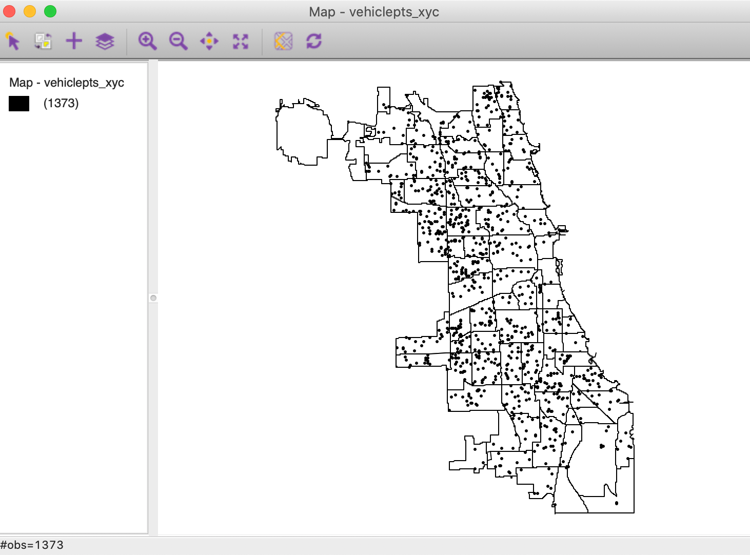
Figure 1: Chicago abandoned vehicles locations
Clustering on Geographical Coordinates
Principle
Applying classic cluster methods to geographical coordinates results in clusters as regions in space. There is nothing special to this type of application. In fact, we have already seen several instances of this in previous chapters, such as the illustrations using the seven point toy example and spectral clustering applied to the canonical spirals data set. In addition, we also applied k-means clustering to MDS coordinates.
When using actual geographical coordinates, it is important to make sure that the Transformation is set to Raw. This is to avoid distortions in the distance measure that may result from the transformations, such as z-standardize.
For example, in the case of Chicago, the range of the coordinates in the North-South direction is much greater than the range in the East-West direction. Standardization of the coordinates would result in the transformed values to be more compressed in the North-South direction, since both transformed variables end up with the same variance (or range). This will directly affect the resulting inter-point distances used in the dissimilarity matrix.
In addition, it is critical that the geographical coordinates are projected and not simply latitude-longitude. This ensures that the Euclidean distances are calculated correctly. Using latitude and longitude to calculate straight line distance is incorrect.
For most methods, the clusters will tend to result in fairly compact regions. In fact, as we have seen, for k-means the regions correspond to Thiessen polygons around the cluster centers. For spectral clustering, the boundaries between regions can be more irregular. Finally, for hierarchical clustering, the result depends greatly on the linkage method chosen. In most situations, Ward’s and complete linkage will yield the most compact regions. In contrast, single and average linkage will tend to result in singletons and/or long chains of points.
Implementation
The cluster methods are invoked in the standard manner. In our example, the variables are X and Y, and, as mentioned, the Transformation is set to Raw. Note that whenever the coordinates are selected among the variables available in the data table (as we did here), there is no check on whether they are appropriate. In our example, they are.
A common problem is that the coordinates are latitude-longitude, which does not allow for the proper Euclidean distances. On the other hand, this allows the flexibility to select any variable as a coordinate. In the next section, we illustrate a way to make sure that geographical coordinates are projected.
The typical settings are illustrated for the application of k-means in Figure 2. The number of clusters is selected as 6. All other options are kept to their default values.
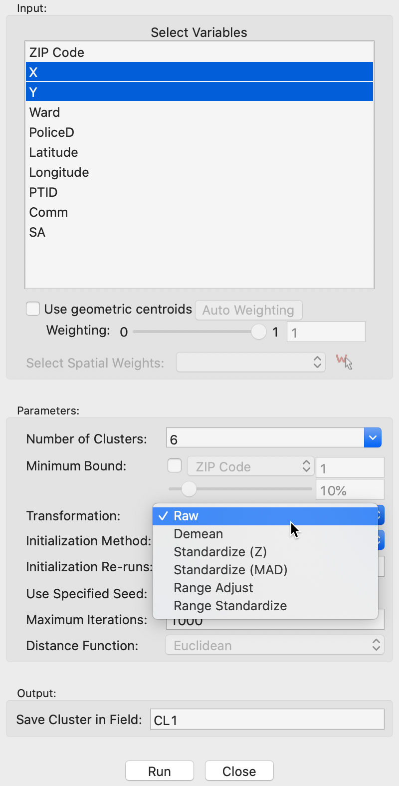
Figure 2: Variable selection – kmeans settings
The resulting cluster maps for four main methods are shown in Figure 3, including k-means, k-medoids, spectral and hierarchical clustering. In each case, the defaults were used, with knn=8 for spectral clustering and Ward’s linkage for hierarchical clustering. The point cluster map is shown on top of the Chicago community area boundaries, in order to highlight the differences between the results.
The colors for the clusters have been adjusted to match the general layout for k-means. While the general organization of the regions is very similar for the four methods, the size of the clusters varies considerably.4
Using the between to total sum of squares as a criterion for comparison, the k-means results are best, with a value of 0.887, but hierarchical clustering is close with 0.878. The values for k-medoids and spectral clustering are slightly worse and almost identical, respectively 0.866 and 0.867 (but keep in mind that this is the wrong criterion to assess k-medoids). K-medoids achieves a reduction of the within distances to 0.337.
It is hard to decide which method works best. K-means will always result in Thiessen polygon like regions, with straight line demarcations between them, which may not necessarily be the desired outcome. Both k-medoids and spectral clustering allow more flexibility in that respect, with k-medoids having an immediate interpretation as the solution to a location-allocation problem. The results for hierarchical clustering vary considerably depending on the linkage method. Strange, string-like regions may follow from the use of methods other than Ward’s or complete linkage in hierarchical clustering.
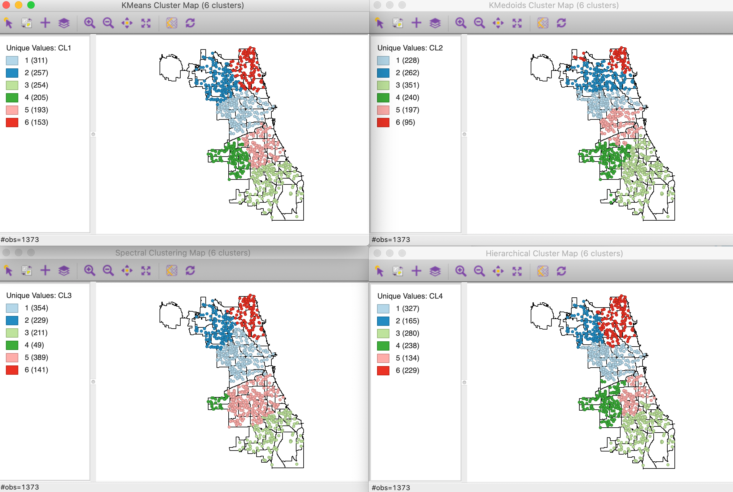
Figure 3: Classic clustering methods applied to point locations
Including Geographical Coordinates in the Feature Set
Principle
As we have seen in the previous chapters, the classic cluster procedures only deal with attribute similarity. They therefore do not guarantee that the resulting clusters are spatially contiguous, nor are they designed to do so. A number of ad hoc procedures have been suggested that start with the original result and proceed to create clusters where all members of the cluster are contiguous. In general, such approaches are unsatisfactory and none scale well to larger data sets.
Early approaches started with the solution of a standard clustering algorithm, and subsequently adjusted this in order to obtain contiguous regions, as in Openshaw (1973) and Openshaw and Rao (1995). For example, one could make every subset of contiguous observations a separate cluster, which would satisfy the spatial constraint. However, this would also increase the number of clusters. As a result, the initial value of k would no longer be valid. One could also manually move observations to an adjoining cluster and visually obtain contiguity while maintaining the same k. However, this becomes quickly impractical when the number of observations is larger.
An alternative is to include the geometric centroids of the observations as part of the clustering process by adding them as variables in the collection of attributes. Early applications of this idea can be found in Webster and Burrough (1972) and Murray and Shyy (2000), among others. However, while this approach tends to yield more geographically compact clusters, it does not guarantee contiguity.
Here again, it is important to ensure that the coordinates are in projected units. Even though it is sometimes suggested in the literature to include latitude and longitude, this is incorrect. Only for projected units are the associated Euclidean distances meaningful.
Also, as pointed out earlier, the transformation of the variables, which is standard in the cluster procedures, may distort the geographical features when the East-West and North-South dimensions are very different. For a more or less square example like the departments in France in the Guerry data set, this is likely a minor issue, but for elongated geographies, such as the state of California or even Chicago, a standardization to a common range will give more importance to the shorter dimension. Due to the standardization, smaller distances in the shorter dimension will have the same weight as larger distances in the longer dimension, since the latter are more compressed in the standardization.
Unlike what we pursued when clustering solely on geographic coordinates, keeping all the variables (including the non-geographical attributes) in a Raw format is not advisable.
Implementation
We start any clustering procedure in the usual fashion, either from the toolbar icon or from the Clusters menu. For this example, we will switch to the Guerry data set. We will use the same four methods as in the previous section: Kmeans, Kmedoids, Spectral, and Hierarchical.
Standard solution
In order to provide a frame of reference, we first carry out the four cluster methods on the original six variables. We select them from the Input panel as Crm_prs, Crm_prp, Litercy, Donatns, Infants and Suicids. In this example, we set k to 4.
For each method, we use the default settings. For spectral clustering, we set the parameter knn to 5 for the best result. To keep track of the various cases, we make sure to set the cluster Field name to something different in each instance (here, we simply use CL1, CL2, CL3 and CL4).
The four results are summarized in Figure 4. As before, the reference labels are those for k-means, with the other categories adjusted so as to mimic its geographic pattern as closely as possible.
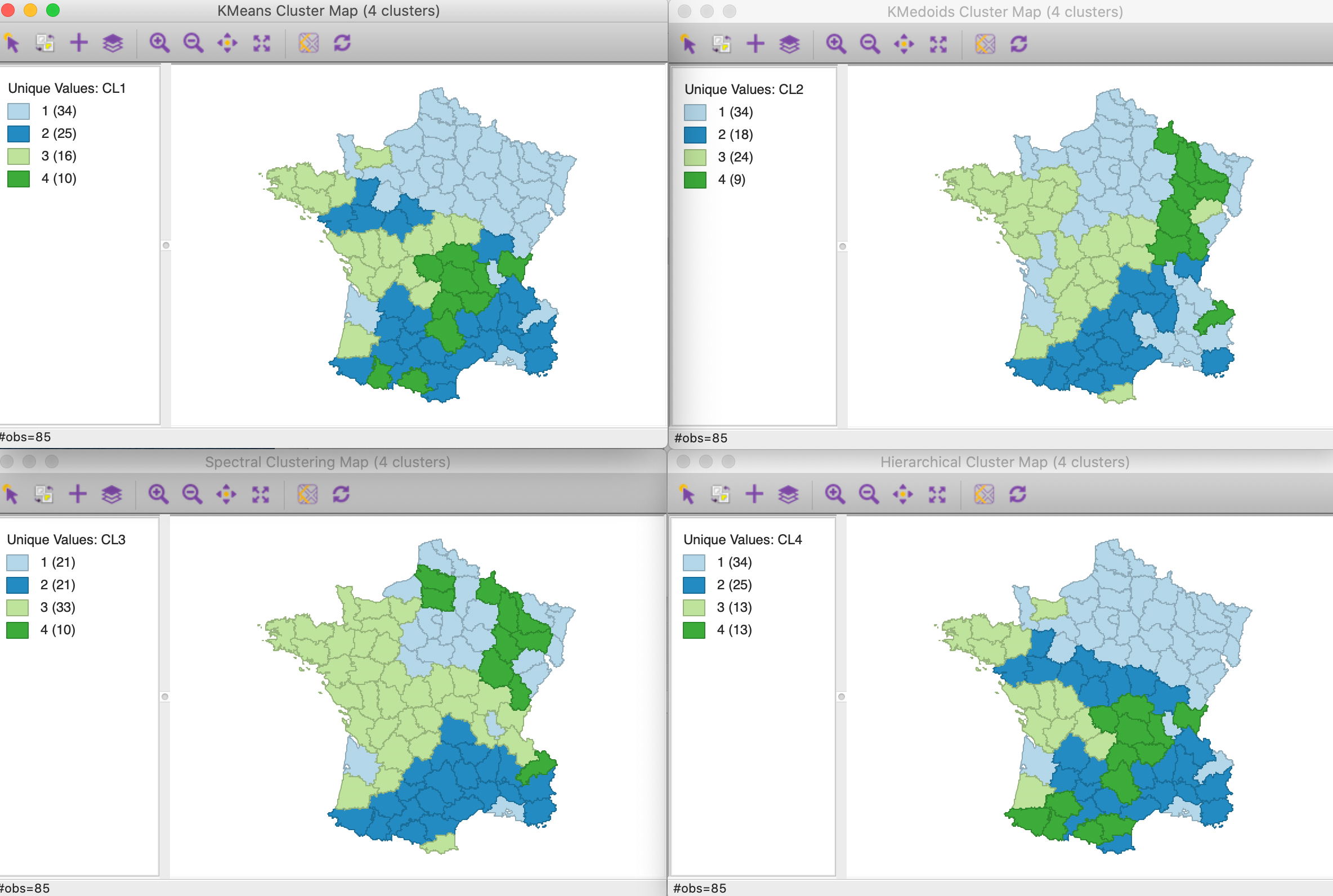
Figure 4: Cluster maps for six variables with k=4
As we have seen before, the results differ by method. In terms of fit, k-means has the best result, with the ratio of between SS to total SS at 0.433. K-medoids achieves 0.369 (but this is not the proper performance measure for k-medoids), spectral 0.376, and hierarchical 0.420.
The geographic grouping of the observations that are part of each cluster is far from contiguous. Typically, there are one or two clusters that come close, but all have some remote disconnected parts. The other clusters are more fragmented spatially.
Solutions with x-y coordinates included
We now repeat the process, but include the two centroids among the attributes of the cluster analysis. In order to make sure that the geographical coordinates are checked for validity, we need to select the variables from the list as <X-Centroids> and <Y-Centroids>, as shown in Figure 5.
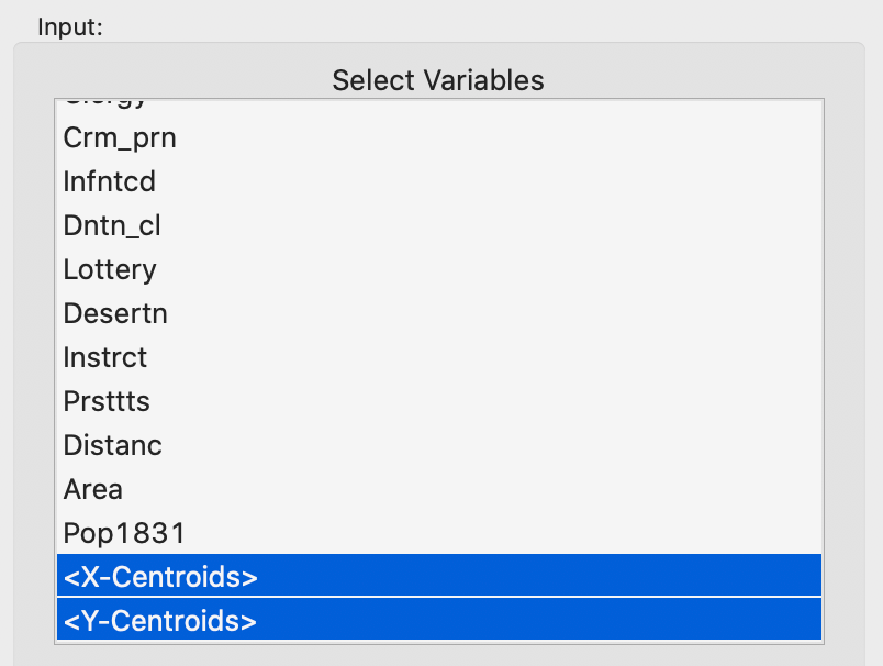
Figure 5: Centroids included in feature set
When we select these reserved variable names from the table, GeoDa carries out a check of the
validity
of the projection. If the coordinates are detected to be decimal degrees (lat-lon) or when no projection
information
is available, a warning is given, as in Figure 6. If one is sure that
the coordinates
are in the proper projection, one can proceed anyway, but any use of latitude-longitude pairs will lead to
incorrect results.
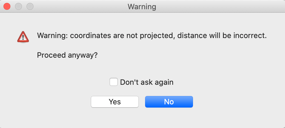
Figure 6: Warning for projection issues
As in the previous application, we set k=4, and keep all other default settings (for spectral clustering, we now select knn=2 for the best result).
The results for the four methods are shown in Figure 7. While not achieving completely contiguous clusters, the spatial layout is much more structured than in the base solutions. In terms of overall fit, again we have the highest between SS to total SS ratio for k-means (0.458), followed by hierarchical clustering (0.445), k-medoids (0.411), and spectral clustering (0.402). Note that this measure now includes the geometric coordinates as part of the dissimilarity measure, so the resulting ratio is not really comparable to the base case.
For all but hierarchical clustering, two of the four clusters are contiguous, with a third missing only one or two observations, and the fourth more spatially scattered. For hierarchical clustering, only one grouping is contiguous, two almost and a fourth is more scattered.
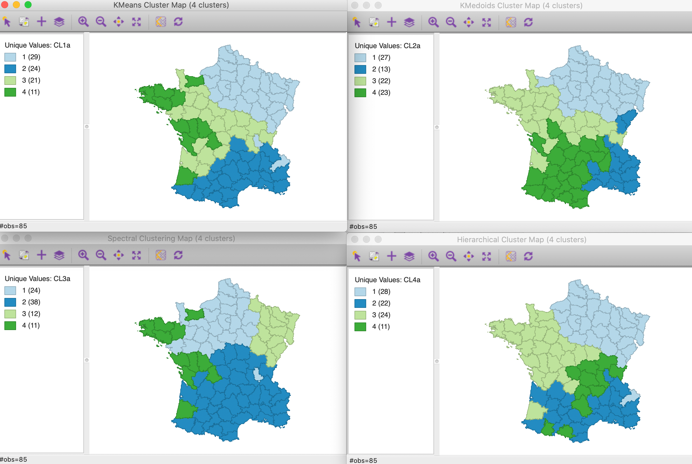
Figure 7: Cluster maps for six variables and x-y coordinates with k=4
The results illustrate that including the coordinates does provide a form of spatial forcing, albeit imperfect. The outcome varies by method and depends on the number of clusters specified (k), as well as the number of attribute variables. In essence, this method gives equal weight to all the variables, so the higher the attribute dimension of the input variables, the less weight the spatial coordinates will receive. As a consequence, less spatial forcing will be possible.
In the next method, the relative weighting of attribute variables relative to geographic variables is made explicit.
Weighted Optimization of Attribute and Geographical Similarity
Principle
When including geographic coordinates among the variables in a clustering excercise, each variable is weighted equally. In contrast, in a weighted optimization, the coordinate variables are treated separately from the regular attributes, in the sense that we can now think of the problem as having two objective functions. One is focused on the similarity of the regular attributes (in our example, the six variables), the other on the similarity of the geometric centroids. A weight changes the relative importance of each objective.
Early formulations of the idea behind a weighted optimization of geographical and attribute features can be found in Webster and Burrough (1972), Wise, Haining, and Ma (1997), and Haining, Wise, and Ma (2000). More recently, some other methods that have a soft enforcing of spatial constraints can be found in Yuan et al. (2015) and Cheruvelil et al. (2017), applied to spectral clustering, and in Chavent et al. (2018) for hierarchical clustering. In these approaches a relative weight is given to the dissimilarity that pertains to the regular attributes and one that pertains to the geographic coordinates. As the weight of the geographic part is increased, more spatial forcing occurs.
The approach we outline here is different, in that the weights are used to rescale the original variables in order to change the relative importance of attribute similarity versus locational similarity. This is a special case of weighted clustering, which is an option is several of the standard clustering implementations. The objective is to find a contiguous solution with the smallest weight given to the x-y coordinates, thus sacrificing the least of attribute similarity.
Let’s say there are \(p\) regular attributes in addition to the x-y coordinates. With a weight of \(w_1 \leq 1\) for the geographic coordinates, the weight for the regular attributes as a whole is \(w_2 = 1 - w_1\). These weights are distributed over the variables to achieve a rescaling that reflects the relative importance of space vs attribute.
Specifically, the weight \(w_1\) is allocated to x and y with each \(w_1/2\), whereas the weight \(w_2\) is allocated over the regular attributes as \(w_2/p\). For comparison, and using the same logic, in the previous method, each variable was given an equal weight of \(1/(p+2)\). In other words, all the variables, both attribute and locational were given the same weight.
The rescaled variables can be used in all of the standard clustering algorithms, without any further adjustments. One other important difference with the previous method is that the x-y coordinates are not taken into account when assessing the cluster centers and performance measures. These are based on the original unweighted attributes.
While the principle behind this approach is intuitive, in practice it does not always work, since the contiguity constraint is not actually part of the optimization process. Therefore, there are situations where simple re-weighting of the spatial and non-spatial attributes does not lead to a contiguous solution.
For all methods except spectral clustering, there is a direct relation between the relative weight given to the attributes and the measure of fit (e.g., between to total sum of squares). As the weight for the x-y coordinates increases, the fit on the attribute dimension will become poorer. However, for spectral clustering, this is not necessarily the case, since this method is not based on the original variables, but on a projection of these (the principal components).
In other words, the x-y coordinates are used to pull the original unconstrained solution towards a point where all clusters consist of contiguous observations. Only when the weight given to the coordinates is small is such a solution still meaningful in terms of the original attributes. A large weight for the x-y coordinates in essence forces a contiguous solution, similar to what would follow if only the coordinates were taken into account. While this obtains contiguity, it does not provide a meaningful result in terms of attribute similarity.
Optimization
The spatial constraint can be incorporated into an optimization process. This approach exploits a bisection search to find the cluster solution with the smallest weight for the x-y coordinates that still satisfies a contiguity constraint. In most instances, this solution will also have the best fit of all the possible weights that satisfy the constraint. For spectral clustering, the solution only guarantees that it consists of contiguous clusters with the largest weight given to the original attributes.
One limitation of this approach is that it does not deal well with islands, or disconnected observations. Consequently, only results that designate the island(s) as separate clusters will meet the contiguity constraint. In such instances, it may be more practical to remove the island observations before carrying out the analysis.
The earlier methods
allow soft spatial clustering, in the sense that not all clusters consist of spatially
contiguous observations. In contrast, the approach outlined here enforces a hard spatial
constraint, although possibly at
the expense of a poor clustering performance for the attribute variables. This method is original to
GeoDa.
The point of departure is a purely spatial cluster that assigns a weight of \(w_1 = 1.0\) to the x-y coordinates. Next, \(w_1\) is set to 0.5 and the contiguity constraint is checked. As customary, contiguity is defined by a spatial weights specification. The spatial weights are represented internally as a graph. For each node in the graph, the algorithm keeps track of what cluster it belongs to.
In order to check whether the elements of a cluster are contiguous, an efficient breadth first algorithm is implemented of complexity O(n). It starts at a random node and identifies all of the neighbors of that node that belong to the same cluster. Technically, the node IDs are pushed onto a stack. In this process, neighbors that are not part of the same cluster are ignored (i.e., they are not pushed onto the stack). Each element on the stack is examined in turn. If it has neighbors in the cluster that are not yet on the stack, they are added. Otherwise, nothing needs to be changed. After this evaluation, the node is popped from the stack. When the stack is empty, this means that all contiguous nodes have been examined. If at that point, there are still unexamined observations in the cluster, we can conclude that the cluster is not contiguous and the process stops. In general, the examination of nodes is carried out until contiguity fails. If all nodes are examined without a failure, all clusters consist of contiguous nodes (according to the definition used in the spatial weights specification). Since the algorithm is linear in the number of observations, it scales well.
To illustrate this process, consider the partial connectivity graph in Figure 8. It only pertains to the connections for the observations in cluster 4 (dark green on the map). The cluster consists of 11 observations, distributed among four spatial units. If we would (randomly) select either of the singletons, the check would be completed immediately, since those observations only have connections to locations outside the cluster. Since 10 remaining observations have not been visited, the cluster is clearly not contiguous.
The process is only slightly more complex if we start with an observation from one of the other two groups, one consisting of four observations, the other of five. In each instance, once the connections to the within group members have been checked, it is clear that the set of 11 observations has not be exhausted, so that the contiguity constraint fails.
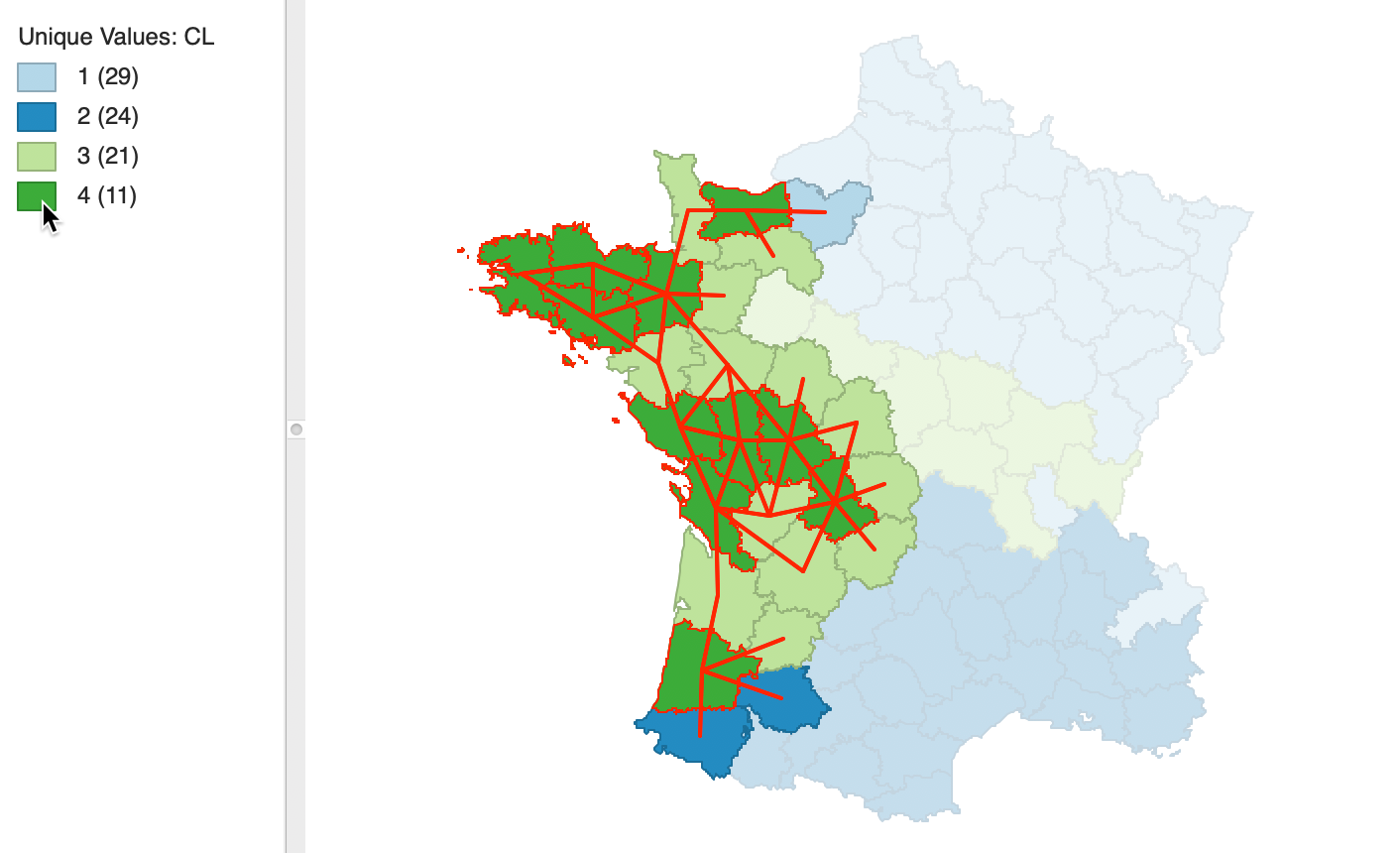
Figure 8: Check on contiguity constraint using connectivity graph
If the contiguity constraint is satisfied, that means that \(w_1\) can be further decreased, to get a better fit on the attribute clustering. Using a bisection logic, the weight is set to 0.25 and the contiguity constraint is checked again.
In contrast, if the contiguity constraint is not satisfied at \(w_1 = 0.5\), then the weight is increased to the mid-point between 0.5 and 1.0, i.e., 0.75, and the process is repeated. Each time, a failure to meet the contiguity constraint increases the weight, and the reverse results in a decrease of the weight. Following the bisection logic, the next point is always the midpoint between the current value and the closest previous value to the left or to the right.
In an ideal situation (highly unlikely in practice), \(w_1 = 0\) and the original cluster solution satisfies the spatial constraints. In the worst case, the search yields a weight close to 1.0, which implies that the attributes are essentially ignored. More precisely, this means that the contiguity constraint cannot be met jointly with the other attributes. Only a solution that gives all or most of the weight to the x-y coordinates meets the constraint.
In practice, any final solution with a weight larger than 0.5 should be viewed with scepticism, since it diminishes the importance of attribute similarity. Also, it is possible that the contiguity constraint cannot be satisfied unless (almost) all weight is given to the coordinates. This implies that a spatial contiguous solution is incompatible with the underlying attribute similarity for the given combination of variables and number of clusters (k). The spatially constrained clustering approaches covered in later chapters address this tension explicitly.
Implementation
The weighted clustering is invoked in the same manner for each of the five standard clustering techniques. Just below the list of variables is a check box next to Use geometric centroids, as shown in Figure 9. The default value, or rather, starting point, is a weight of 1.0. This corresponds to clustering on the coordinates of the centroids of the spatial units. In contrast to the previous method, the coordinates do not need to be specified in the variable list. They are calculated under the hood. As before, a warning is generated when the projection information is invalid.
In addition, a spatial weights file needs to be specified. This is used to assess the spatial constraint.5 In our example, we use queen contiguity as defined in the guerry_85_q file.
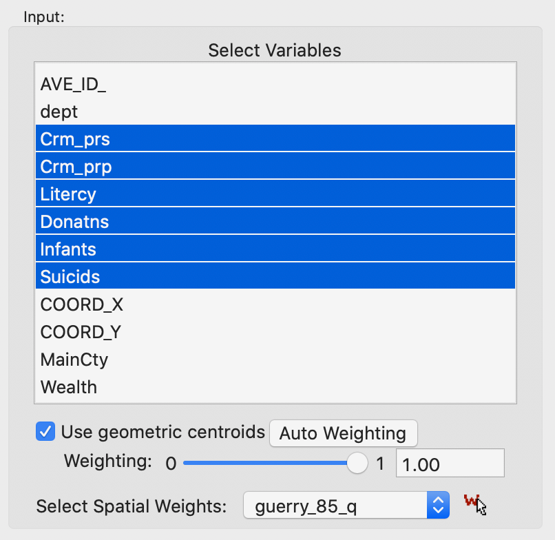
Figure 9: Use Geometric Centroids
As a frame of reference, the cluster map and summaries that result for a pure geometric solution that uses hierarchical clustering with Ward’s linkage are given in Figures 10 and 11. Clearly, contiguity is achieved, but at the expense of a serious deterioration in fit relative to the unconstrained solution. For comparison, the cluster map for the latter can be found in the lower-right panel of Figure 4.
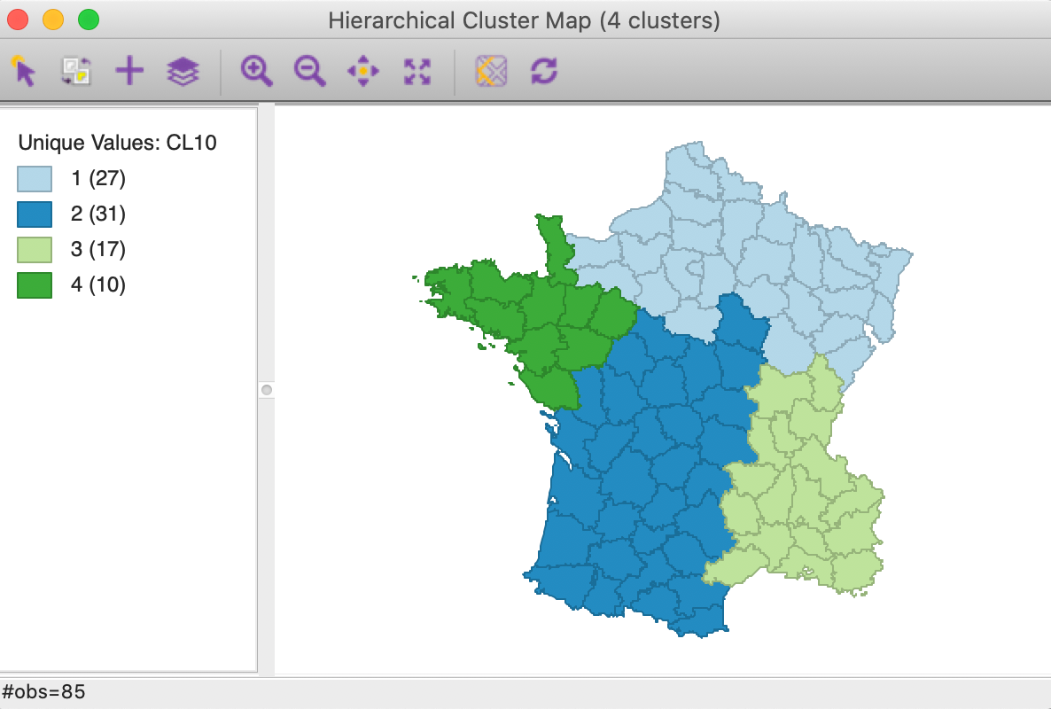
Figure 10: Cluster map - pure geometric solution - Ward’s linkage (k=4)
The ratio of the between to total sum of squares was 0.420 for the unconstrained solution. Here, it is down to 0.266. Note how the summary in Figure 11 shows the weights for both the centroids and the regular attribute variables. However, the cluster centers and summary statistics only take into account the latter. As in the regular case, the centroids are given in the scale of the original variables, whereas the sum of squares are listed for whatever standardization was used (z-standardize in our example).
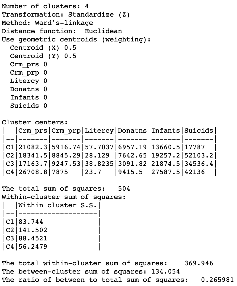
Figure 11: Cluster summary - pure geometric solution - Ward’s linkage (k=4)
Manual specification of weights
Any weight can be specified by typing its value in the box on the interface in Figure 9, or by moving the slider until the desired value is shown. For example, in Figures 12 and 13, the cluster map and cluster summary are shown for a weight of 0.5 (continuing with hierarchical clustering using Ward’s linkage).
In our example, it is possible to check the spatial contiguity constraint visually. In more realistic examples, this will very quickly become difficult to impossible to verify. Here, contiguity is cleary achieved for a weight of 0.5. This suggests that the weight could be further lowered to obtain a better solution (in terms of giving greater weight to the attribute variables).
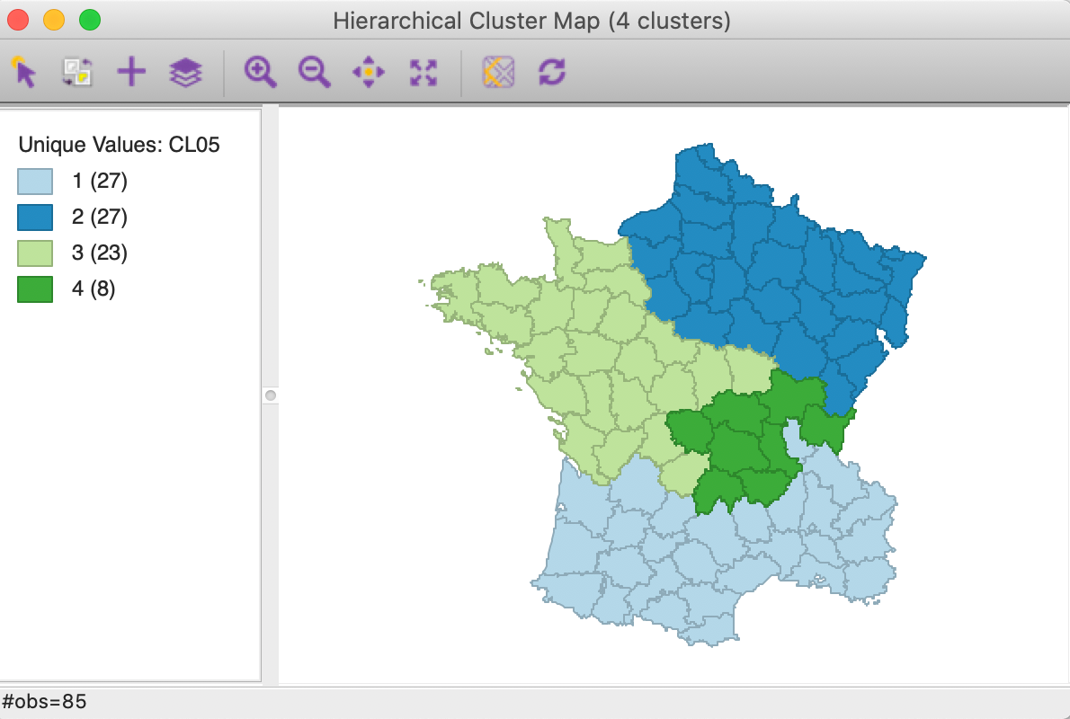
Figure 12: Cluster map - weight = 0.5 - Ward’s linkage (k=4)
The cluster summary shown an improvement of the measure of fit to 0.381 relative to 0.266 for the pure geometric solution, but lower than the 0.420 for the unconstrained solution.
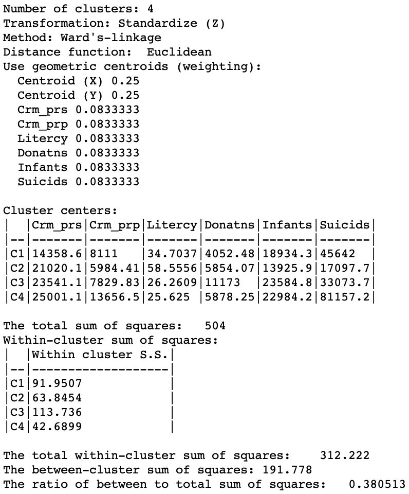
Figure 13: Cluster summary - weight = 0.5 - Ward’s linkage (k=4)
Optimal weights
In our simple example, it is possible to carry out the bisection search manually, by changing the weight at each iteration and visually checking the contiguity constraint. To begin, since the spatial constraint is satisfied for 0.5, we know that the next step is to reduce the weight to 0.25. At this point, the constraint is no longer satisfied (not shown), so that we then have to move to the mid-point between 0.25 and 0.5, or 0.375.
The full set of iterations until convergence at 4 decimal points is listed in Figure 14. In all, it takes 15 steps, at each stage moving left or right depending on whether the constraint is satisfied. In the table, an x in the second column corresponds with meeting the contiguity constraint. The third column indicates the change in the weight. Each time the constraint is met, the adjustment is negative, and the converse holds when the constraint is not met. The iteraction continues until there is no change in the fourth decimal of the weight. In our example, the final solution yields a weight of 0.480042.
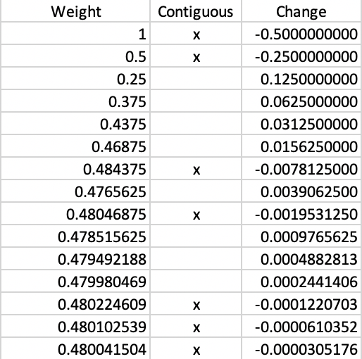
Figure 14: Manual weight iterations - Ward’s linkage (k=4)
Of course, in most realistic applications, it will be impractical to carry out these iterations by hand. By selecting the Auto Weighting button in the interface (shown in Figure 9), the solution to the bisection search is given in the box for the weight.
For the four methods we consider for k=4, this yields 0.45 for k-means, 0.35 for k-medoids, 0.51 for spectral clustering (using knn=5) and 0.48 for hierarchical clustering (using Ward’s linkage). The corresponding cluster maps are shown in Figure 15.
The worst solution is for spectral clustering. Even though the resulting regions are quite compact, this is a reflection of a large weight given to the centroids relative to the regular attributes. The best solution is arguably obtained for k-medoids, with a weight of 0.35, although it is not the best in terms of overall fit (0.336 – albeit on an inappropriate measure). The best solution on the sum of squares criterion is hierarchical clustering, which, as we have seen, achieves 0.381, compared to 0.361 for k-means and 0.266 for spectral clustering.
In general, for smaller values of the weight, a more irregular regionalization occurs, driven to a greater extent by the pure attribute similarity. On the other hand, with the weight around 0.5, the dominant factor becomes the centroids, which is less interesting in terms of attribute clustering.
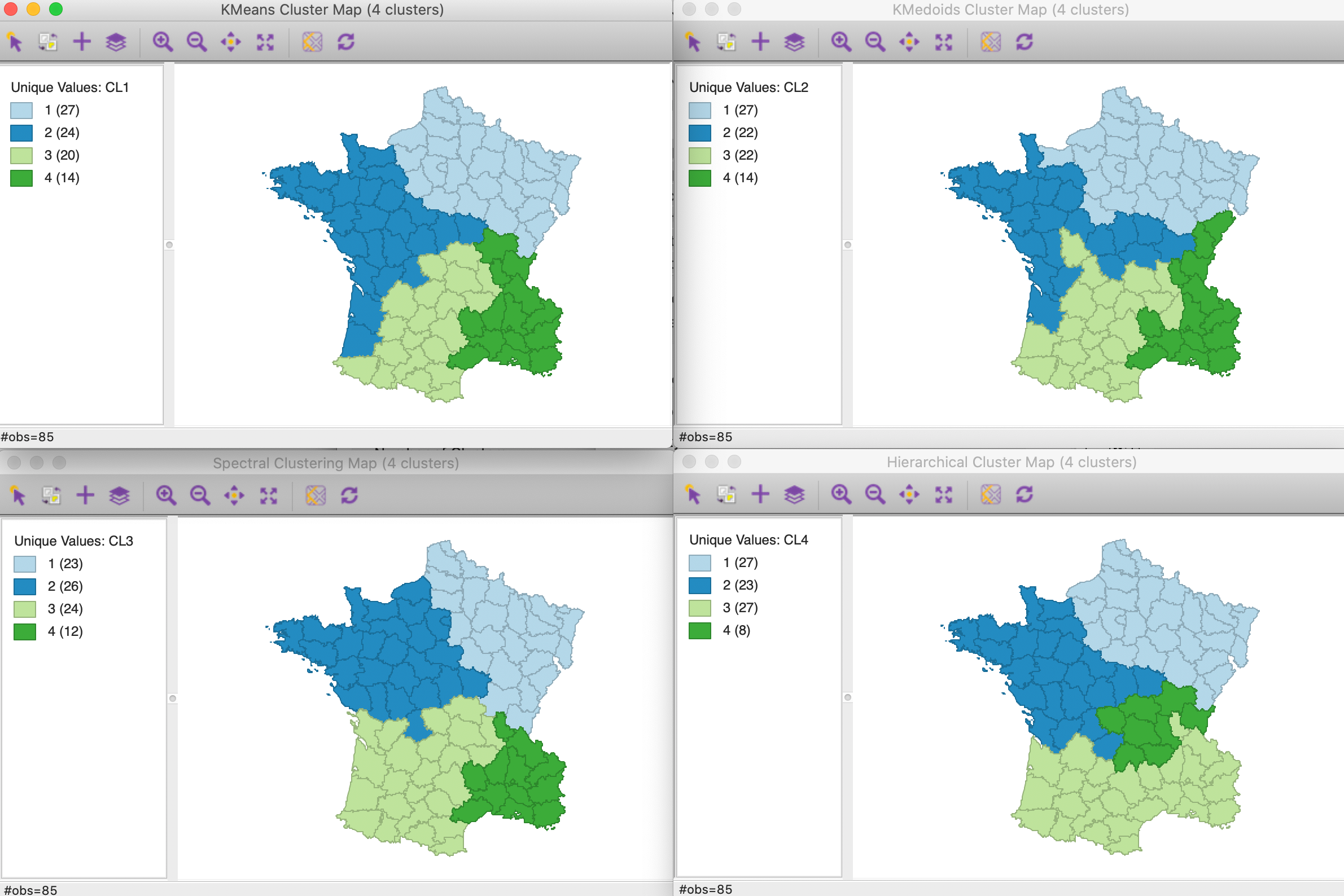
Figure 15: Cluster maps for six variables and optimal weights with k=4
It is important to keep in mind that this approach will not yield satisfactory solutions in many instances in practice. It is primarily included as a pedagogic device, to illustrate the trade offs between attribute and locational similarity. In the methods covered in the following chapters, the spatial aspects of the clustering are taken into account in a fully explicit manner, rather than indirectly as discussed here.
References
Chavent, Marie, Vanessa Kuentz-Simonet, Amaury Labenne, and Jérôme Saracco. 2018. “ClustGeo: An R Package for Hierarchical Clustering with Spatial Constraints.” Computational Statistics 33: 1799–1822.
Cheruvelil, Kendra Spence, Shuai Yuan, Katherine E. Webster, Pang-Ning Tan, Jean-François, Sarah M. Collins, C. Emi Fergus, et al. 2017. “Creating Multithemed Ecological Regions for Macroscale Ecology: Testing a Flexible, Repeatable, and Accessible Clustering Method.” Ecology and Evolution 7: 3046–58.
Haining, Robert F., Stephen Wise, and Jingsheng Ma. 2000. “Designing and Implementing Software for Spatial Statistical Analysis in a GIS Environment.” Journal of Geographical Systems 2 (3): 257–86.
Murray, Alan T., and Tung-Kai Shyy. 2000. “Integrating Attribute and Space Characteristics in Choropleth Display and Spatial Data Mining.” International Journal of Geographical Information Science 14: 649–67.
Openshaw, Stan. 1973. “A Regionalisation Program for Large Data Sets.” Computer Applications 3-4: 136–47.
Openshaw, Stan, and L. Rao. 1995. “Algorithms for Reengineering the 1991 Census Geography.” Environment and Planning A 27 (3): 425–46.
Webster, R., and P. Burrough. 1972. “Computer-Based Soil Mapping of Small Areas from Sample Data II. Classification Smoothing.” Journal of Soil Science 23 (2): 222–34.
Wise, Stephen, Robert Haining, and Jingsheng Ma. 1997. “Regionalisation Tools for Exploratory Spatial Analysis of Health Data.” In Recent Developments in Spatial Analysis: Spatial Statistics, Behavioural Modelling, and Computational Intelligence, edited by Manfred M. Fischer and Arthur Getis, 83–100. New York, NY: Springer.
Yuan, Shuai, Pang-Ning Tan, Kendra Spence Cheruvelil, Sarah M. Collins, and Patricia A. Soranno. 2015. “Constrained Spectral Clustering for Regionalization: Exploring the Trade-Off Between Spatial Contiguity and Landscape Homogeneity.” In 2015 IEEE International Conference on Data Science and Advanced Analytics (DSAA. Paris, France. https://doi.org/10.1109/DSAA.2015.7344878.
-
University of Chicago, Center for Spatial Data Science – anselin@uchicago.edu↩︎
-
This data set is also included as one of the sample data sets on the GeoDaCenter data page.↩︎
-
To obtain the figure as shown, the size of the points was changed to 1pt, their fill and outline color set to black. Similarly, the community area outline color was also changed to black.↩︎
-
Note that only for k-means is the first label associated with the largest clusters. Since
GeoDaorders the labels by cluster size, after the labels are re-arranged, this is no longer necessarily the case.↩︎ -
In the absence of a weights file, a warning is generated.↩︎