Spatial Data Handling
Luc Anselin1
07/21/2018 (updated)
Introduction
In this lab, we will go through some examples of the types of manipulations (data munging or data wrangling) typically required to get your data set ready for analysis. It is commonly argued that this typically takes around 80% of the effort in a data science project (for example, as mentioned in Dasu and Johnson 2003). We will use the City of Chicago open data portal to download data on abandoned vehicles. Our end goal is to create some choropleth maps with abandoned vehicles per capita for Chicago community areas. In order to accomplish this, we will employ functionality in the GeoDa Table and Map commands. Before we can create the maps, we will need to select observations, aggregate data, join different files and carry out variable transformations in order to obtain a so-called “spatially intensive” variable for mapping.
Objectives
After completing the lab, you should know how to carry out the following tasks:
-
Download data from any Socrata-driven open data portal, such as the City of Chicago open data portal
-
Create a GeoDa data table from a csv formatted file
-
Manipulate variable formats, including date/time formats
-
Edit table entries
-
Select observations using the Selection Tool in GeoDa
-
Create a new data layer from selected observations
-
Convert a table with point coordinates to a point layer in GeoDa
-
Spatial selection
-
Spatial aggregation
-
Joining tables
-
Variable calculations in a GeoDa Table
-
Basic choropleth mapping
GeoDa functions covered
- GeoDa > Preferences
- File > Open
- data source connection dialog
- input and output file formats
- CSV input file configuration
- File > Close
- File > Save
- File > Save Selected As
- Table > Edit Variable Properties
- Variable Properties dialog
- Table > Calculator
- Calculator dialog
- Table > Selection Tool
- Selection Tool dialog
- Table > Invert Selection
- Table > Save Selection
- Table > Move Selected to Top
- Table > Merge
- Table Merge dialog
- Table > Delete Variables
- Delete Variable dialog
- Table edits
- Sort table on a variable
- Edit table cells
- Table Aggregate
- Table aggregation dialog
- Tools > Shape > Points from Table
- Table > Points from Table
- Map window toolbar
- Base Map icon and dialog
- Select icon / spatial selection
Obtaining data from the Chicago Open Data Portal
Our first task is to find the data on abandoned vehicles on the data portal and downloading them to a file so that we can manipulate it in GeoDa. The format of choice is a comma delimited file, or csv file. This is basically a spreadsheet-like table with the variables as columns and the observations as rows.
Downloading the data
- Go to the City of Chicago open data portal
The first interface looks like

City of Chicago Open Data Portal
- Select the button for Service Requests. This contains a list of different types of 311 nuisance calls, as shown in
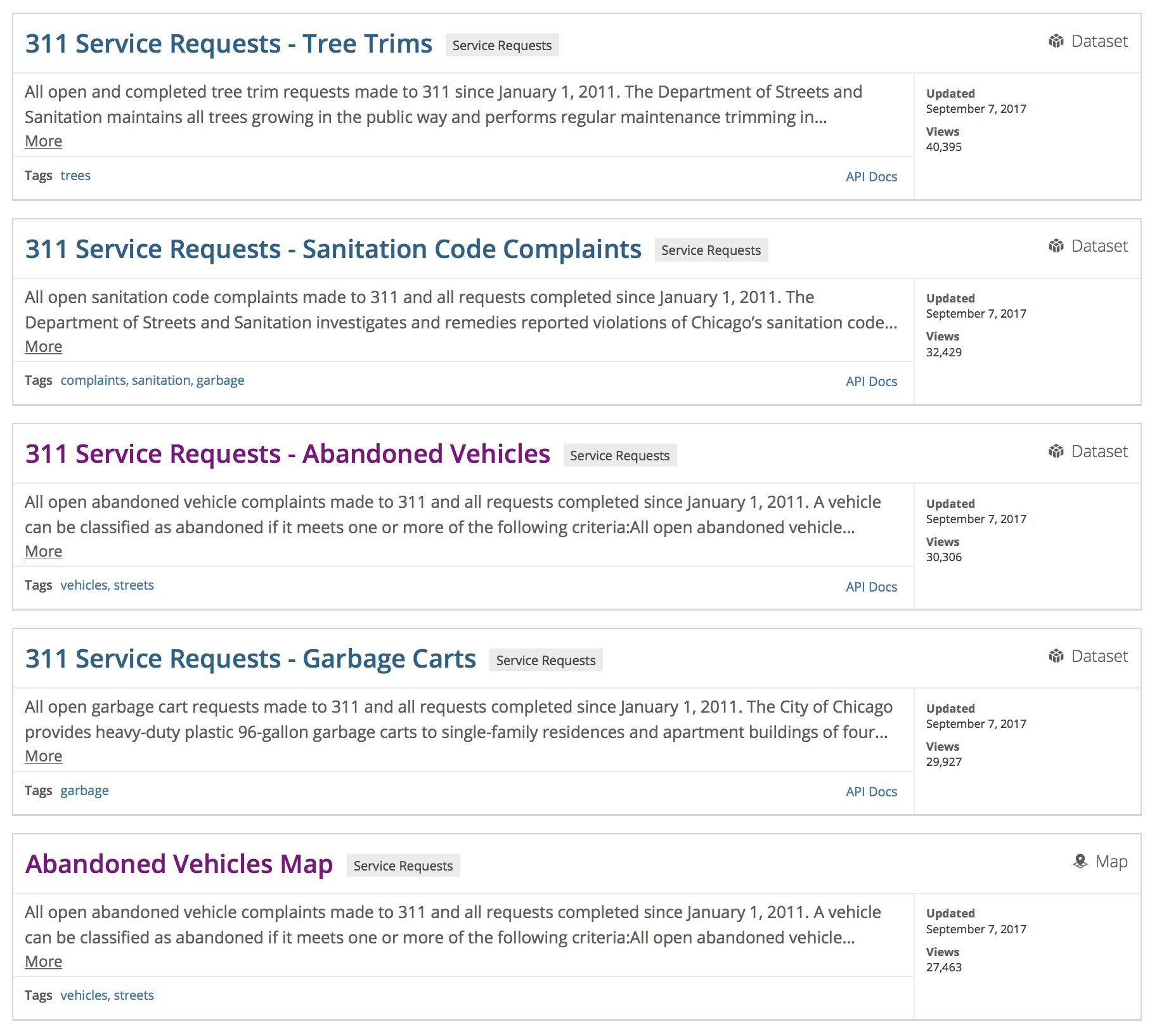
City of Chicago Service Requests
- Scroll down the list and pick 311 Service Requests - Abandoned Vehicles. A brief description of the data source is provided, as shown in

311 Requests for Abandoned Vehicles
Your description may differ slightly, the figure above was created on September 7, 2017.
- To download the data, select the Download button and choose CSV from the drop down list, as shown below:
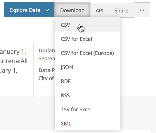
Download CSV Format
The file will be downloaded to your drive. Note: this is a very large file with 22 columns and 172K rows!
You can now open this file in a spreadsheet to take a look at its contents (alternatively, you can also open it in any text editor). The top few rows will look like the figure below:
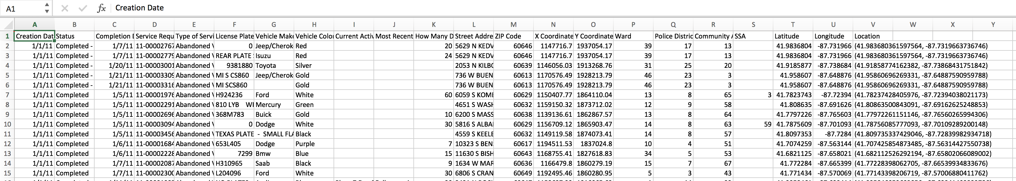
Abandoned Vehicles CSV File Contents
Inspecting the cells, you see that there are many empty ones and the coding is not entirely consistent. We will deal with this by selecting only those variables/columns that we are interested in and only taking a subset of observations for a given time period, in order to keep things manageable.
Online map of the abandoned vehicles
- An alternative approach would be to select the Abandoned Vehicles Map item instead. This defaults to a map of the abandoned vehicle locations, as shown below:
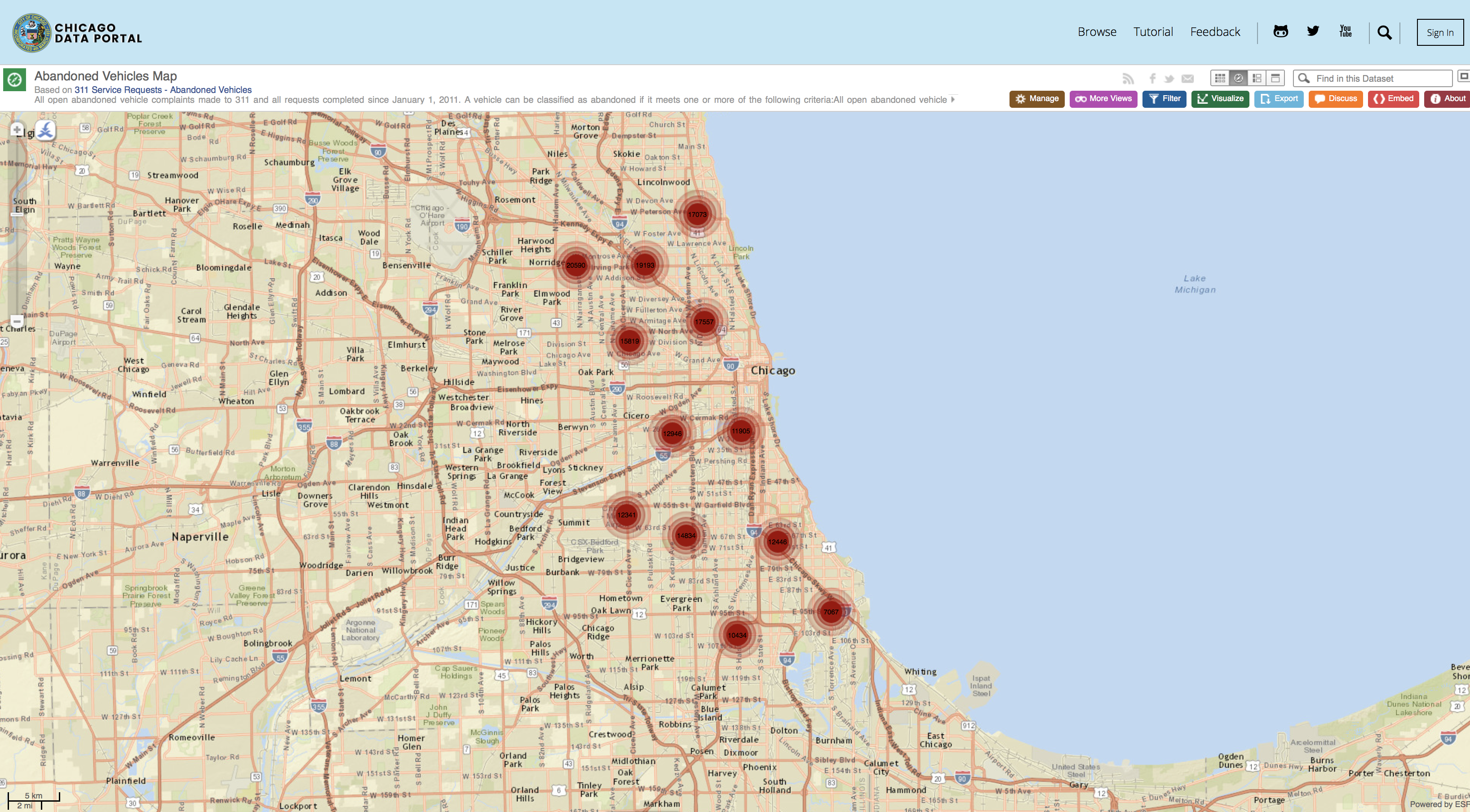
Abandoned Vehicles Default Map
You can get further detail by zooming in on the map, for example, for the Midway in Hyde Park, it will look something like the figure below:
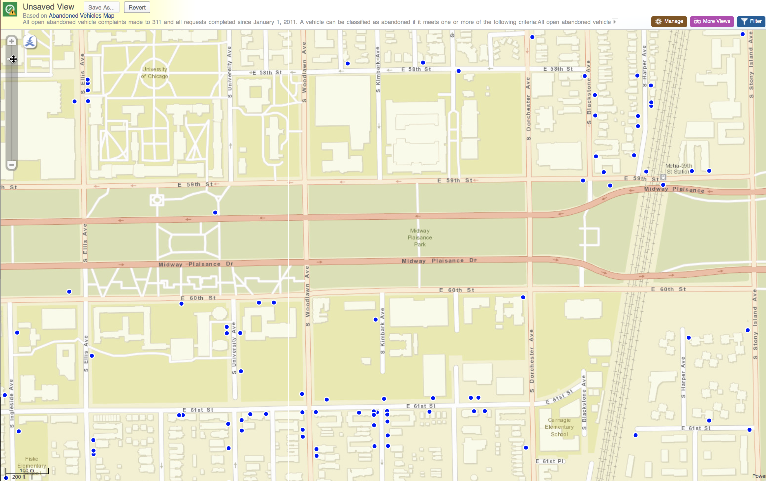
Abandoned Vehicles Close Up Map – Hyde Park Midway
We will not further pursue this at this point, and return to mapping later. An alternative way to download the csv file would be to use the CSV format from the Export button on the upper right hand side of the map, as shown:
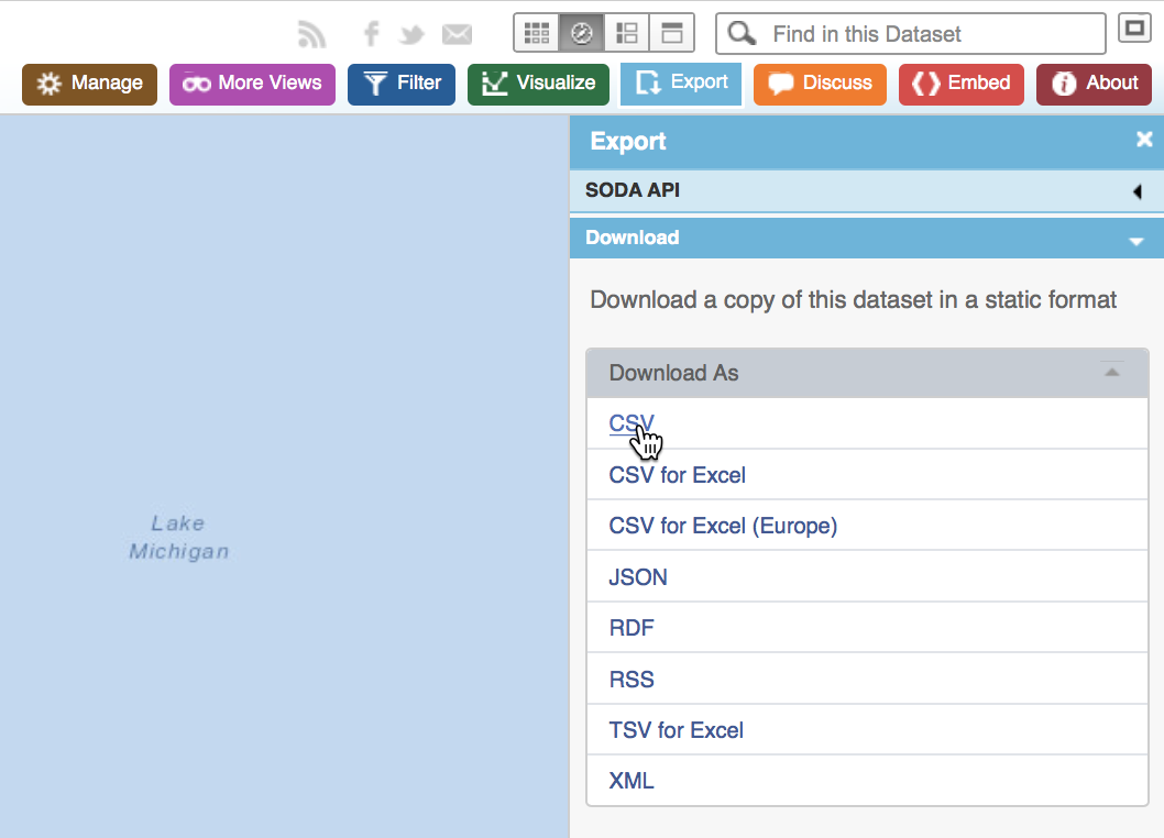
Export from Abandoned Vehicles Map
Selecting Observations for a Given Time Period
For the sake of this exercise, we don’t want to deal with all observations. Instead, say we are interested in analyzing the abandoned vehicle locations for a given time period, such as the month of September 2016. To get to this point, we will need to move through the following steps:
-
import the csv file into GeoDa
-
convert the date stamp into the proper Date/Time format
-
extract the year and month
-
select those observations for the year and month we want
-
keep only those variables/columns of interest to us
This will involve various functionalities of the GeoDa Table, such as the variable properties editor, the Preferences setting, the Calculator, the Selection Tool, and the option to delete variables. The end result will be a table saved in the dbf format (parenthetically illustrating the use of GeoDa as a format converter).
Loading the data
The first step is to load the data from the csv file into GeoDa. After launchig GeoDa, the Connect to Data Source dialog should open. If you do not start GeoDa from scratch, make sure to select the Open icon from the toolbar (the left-most icon).
Open Toolbar Icon
Next, we drag the file 311_Service_Requests-Abandoned_Vehicles.csv (or its equivalent, if you renamed the file) into the Drop files here box of the data dialog, as shown below:
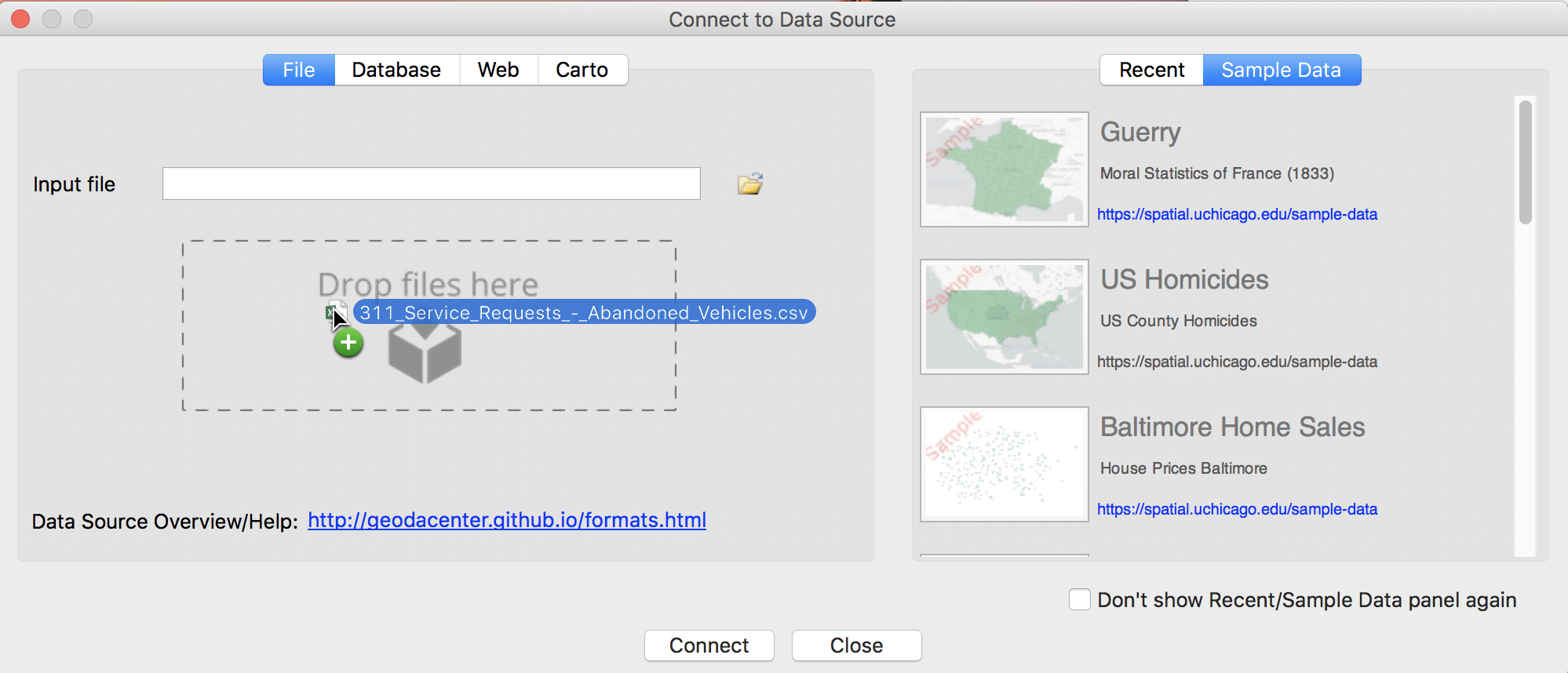
CSV Data Import
Note how the data entry dialog contains several sample data sets (under the tab Sample Data) that can be loaded by a simple click. Also, as soon as you start working with a data set of your own, it will be included in the list under the Recent tab.
Since the csv format is a simple text file without any metadata, there is no way for GeoDa to know what type the variables are, or other such characteristics of the data set. To set some simple parameters, the CSV File Configuration dialog pops up:
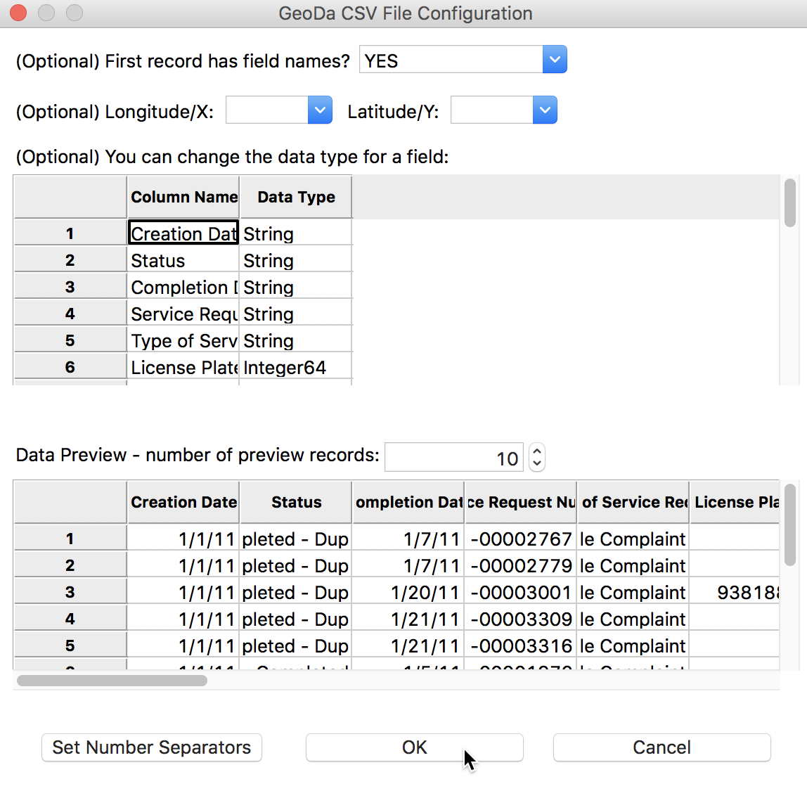
CSV File Configuration
The program tries to guess the type for the variables, but mostly treats them as String. We will deal with this later. For now, make sure the First record has field names item is set to YES (the default setting), and leave all other options as they are. After clicking the OK button, the data table will show the contents of the file, with the number of observations (172326) in the status bar at the bottom.
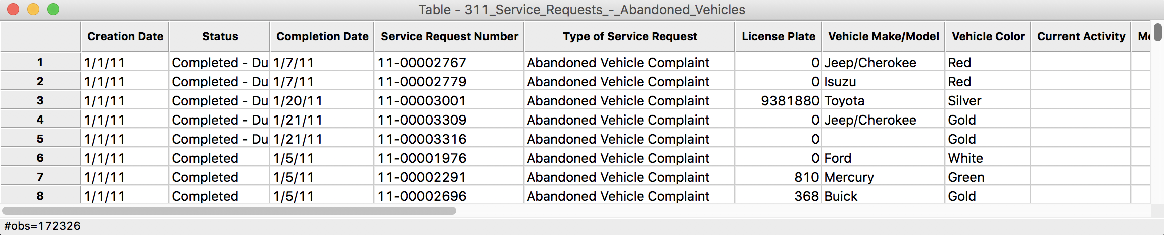
Table Contents
Converting a string to date format
We want to select the observations for the month of September in 2016. Before we can create the query, we need to transform the Creation Date to something manageable that we can search on. As it stands, the entries are in string format (sometimes also referred to as character format). We can check this by means of the Edit Variable Properties option in the Table menu. You access this from the menu (Table > Edit Variable Properties) or by right-clicking in the Table itself, which brings up the menu options.
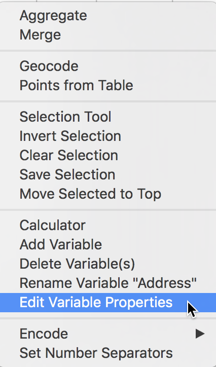
Table Options
A cursory inspection of the type shows the Creation Date to be string. This is not what we want, so we click on the string item and select date from the drop down list.
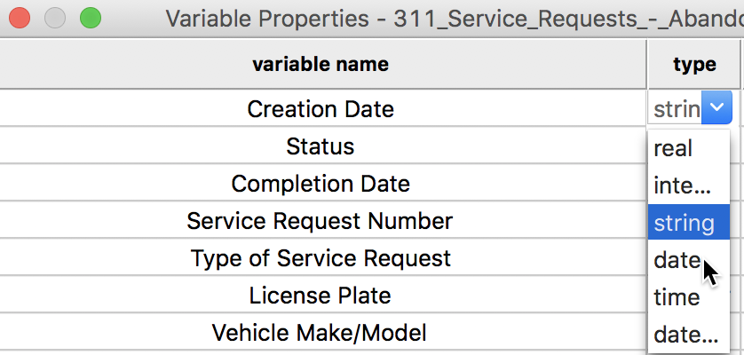
Editing the Variable Type
But what happens? We get an error message (there is no data science project without its share of error messages and other gotchas):
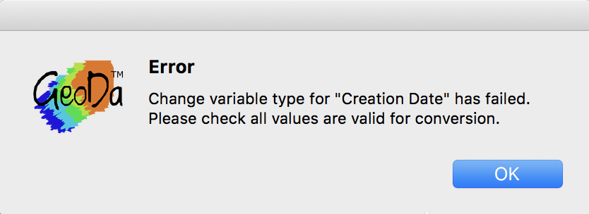
Date Type Error Message
The current functionality to manipulate dates and times in GeoDa is limited to a small set of commonly used default formats. However, the format used in the Abandoned Vehicles data set does not conform to any one of these (hence the error message). So, we need to enter it explicitly into the Preferences pane. Close the variable properties dialog and then, from the main menu, select GeoDa > Preferences to bring up the Preferences pane.
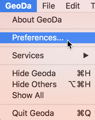
GeoDa Preferences Settings
In the Preferences pane, select the Data Source tab, which will show the current settings. Note the various default formats for Date and Time settings. These use %m for the month, %d for the day and %y for the year (%Y for the year in full four digits).
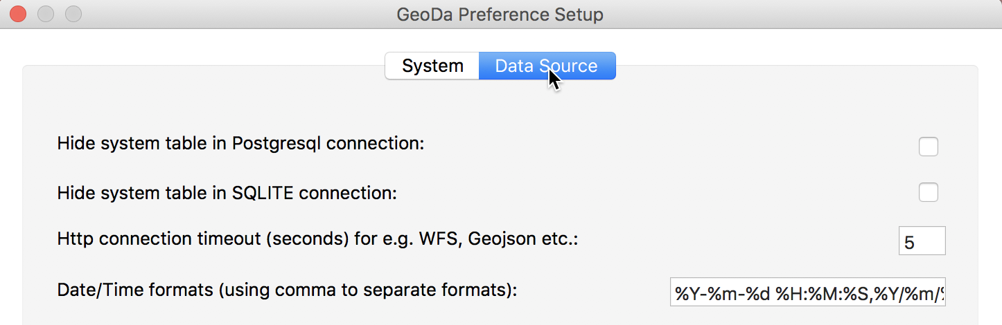
Preferences for Data Sources
In order for GeoDa to recognize dates such as 1/1/11, we need to enter %m/%d/%y into the options box, as shown below.

New Date Setting
We can now go back to the Edit Variable Properties dialog and change the type of the Creation Date to date, as originally intended. Now, everything works as advertised.
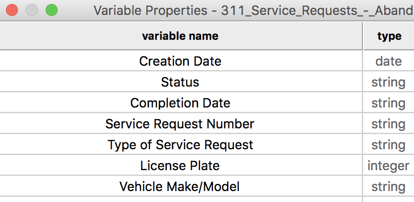
Creation Date as Date Type
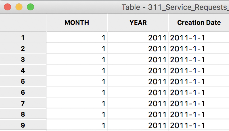
In the data table, the previous entries of 1/1/11, etc., are now replaced by a proper date format, e.g., 2011-1-1, as in:
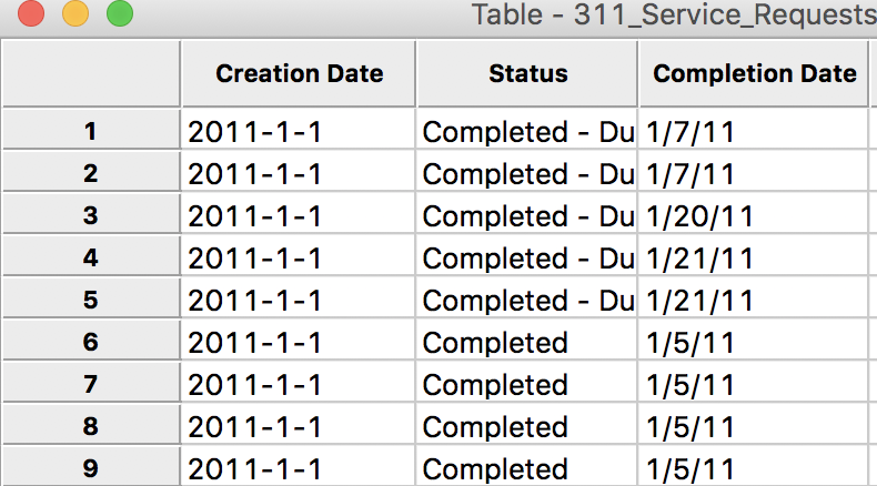
Creation Date in Table
Extracting month and year from the date format
Currently, search functionality on date formats is not implemented in GeoDa. But we can extract the year and month as integer and then use those in the Table Selection Tool. In order to get the year and month, we need to use the Calculator item in the Table menu. Select Table > Calculator or choose this item in the Table option menu (right click in the table).
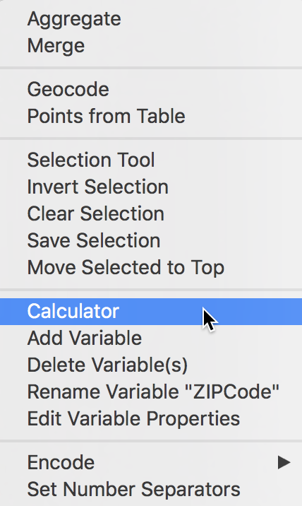
Calculator Option
This brings up the Calculator dialog:
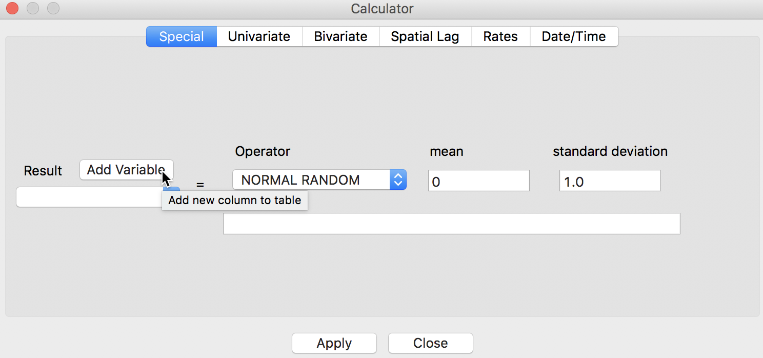
Calculator Dialog
The creation of new or transformed variables operates in two steps:
-
add a new variable (place holder for the result) to the table
-
assign the result of a calculation to the new variable
You can also assign the results of a calculation to an existing variable (instead of creating a new one), but this can be very dangerous. It is much better practice to create a new variable and then delete the one you want to have replaced (after these steps, you can optionally change the name of the newly created variable to the name of the one you deleted).
The types of calculations are given in the tabs at the top of the dialog. At this point, GeoDa supports:
-
Special operations, such as random variable computation and the creation of a simple sequence number (enumerate)
-
Univariate operations, such as assigning a constant, changing the sign, standardize the variable, or randomly reshuffling the observations (shuffle)
-
Bivariate operations, including all standard arthmetic operations
-
Spatial Lag, the creation of spatially lagged variables (using a given spatial weights matrix)
-
Rates, the computation of rates or proportions and associated smoothing methods
-
Date/Time, the manipulation of the contents of a date/time object, such as extracting the month or the year
We will use the right-most tab to create a new integer variable for the year and for the month. First, we select Add Variable to bring up a dialog to specify the properties of the new variable. For example, we can set YEAR to be an integer variable. We can also specify where in the table we want the new column to appear. The default is to put it to the left of the first column, which we will use here. But you can also add it at the end of the columns, or insert anywhere specified in front (i.e., to the left) of a given field.
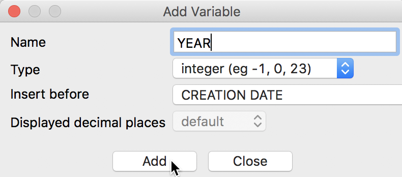
Add Variable Dialog
After pressing the Add button, a new empty column (holding the values 0) will be added to the data table. Now, we go back to the Calculator dialog. We specify the new variable YEAR as the outcome variable for the operation and select Get Year from the Operator drop down list. The Variable/Constant should be set to Creation Date.
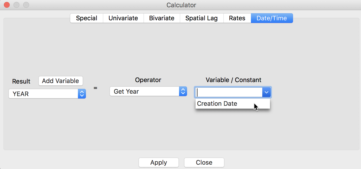
Extract Year
After clicking on Apply, an integer with the value for the year will be inserted in the YEAR column of the table. We proceed in the same fashion to create a variable MONTH and then use Get Month to extract it from the Creation Date. After these operations, there are two new columns in the data table, respectively containing the month and the year.
Month and Year in Data Table
Extracting observations for the desired time period
We now have all the elements in place to design some queries to select the observations for the month of September 2016 (or any other time period). We invoke the Table Selection Tool from the main menu, as Table > Selection Tool, or from the options menu by right-clicking on the table.
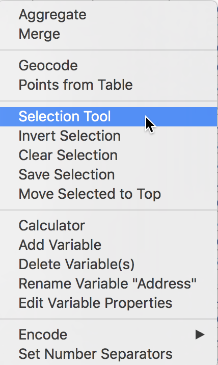
Selection Tool
This brings up the Selection Tool dialog. We proceed in two steps. First, we select the observations for the year 2016, then we select from that selection the observations for the month September. The first query is carried out with the New Selection radio button checked, and YEAR as the Selection Variable. We specify the year by entering 2016 in both boxes for the <= conditions. Then we click on Select All in Range. The selected observations will be highlighted in yellow in the Table (since this is a large file, you may not see any yellow observations in the current table view – as we will see later, you can bring the selected observations to the top by choosing Move Selected to Top from the Table menu). The number of selected observations will be listed in the status bar. In this example, there were 32,822 abandoned vehicles in Chicago in 2016.
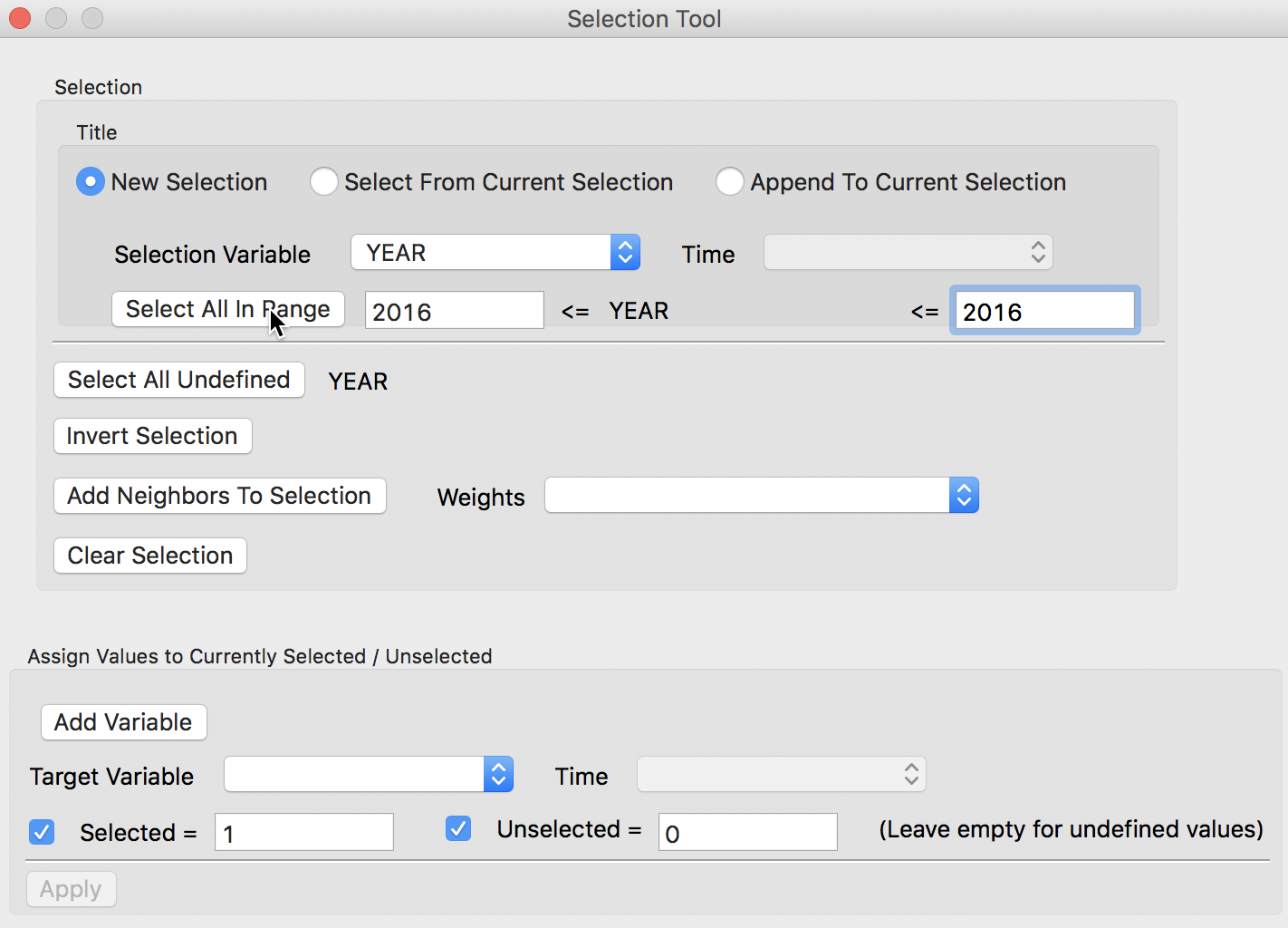
Select Year
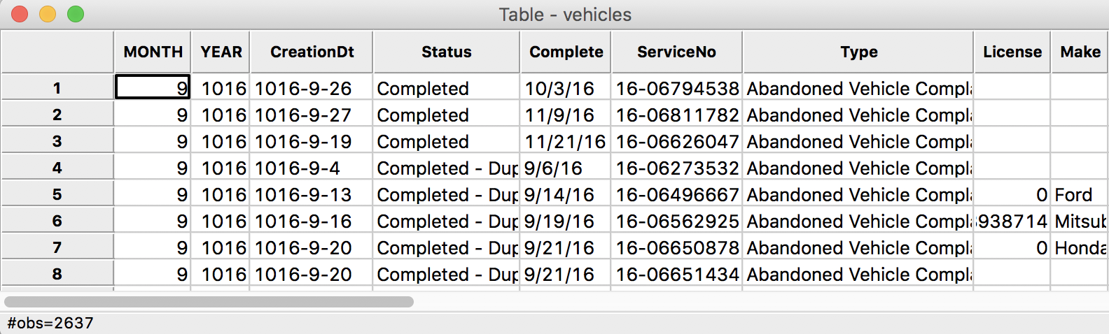
For the second query, we check the radio button for Select From Current Selection and now specify MONTH as the Selection Variable. We enter 9 in the selection bounds boxes and again click on Select All in Range. The selected observations will now be limited to those in 2016 and in the month of September. Again, the corresponding lines in the table will be highlighted in yellow, and the size of the selection given in the status bar. In this case, there were 2,637 abandoned vehicles.
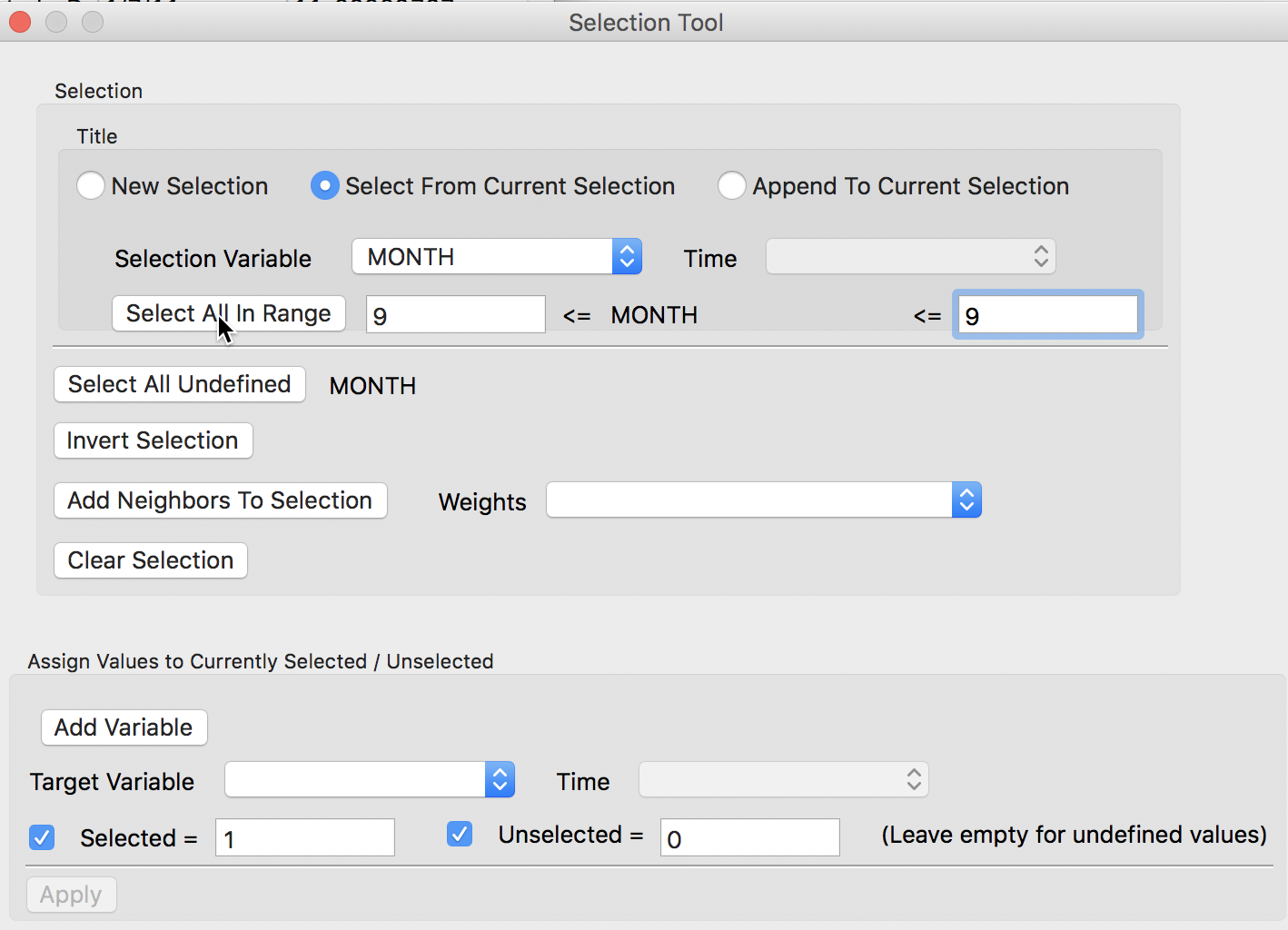
Select Month From Selection
Saving the data in a different format
So far, all operations have been carried out in memory, and if we close GeoDa, all the changes will be lost. In order to make them permanent, we need to save the file. We use this as an opportunity to illustrate the powerful format conversion functionality in GeoDa. While we initially read the data from a CSV file, we will save the selected observations as a new table in the DBF format.
In order to start this process, we first select Save Selected As from the File menu, as File > Save Selected As.
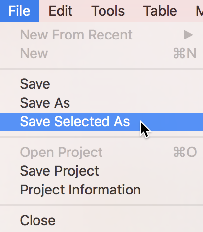
Save Selected As
This brings up a file dialog. Click on the file folder icon to bring up a list of possible output file formats. Now we select dBase Database File, as shown.
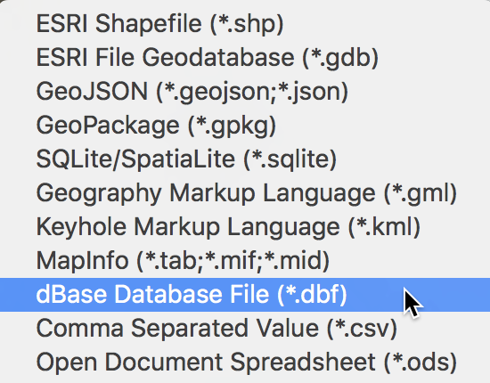
Save As DBF File
We specify the filename as vehicles.dbf, but before the file can be saved, there is a minor problem. The DBF file format is extremely picky about variable names (e.g., no more than 10 characters, no spaces) and several of the variable names from the Chicago Open Data Portal do not conform to this standard. GeoDa flags the violating variable names and suggests new field names, as shown.
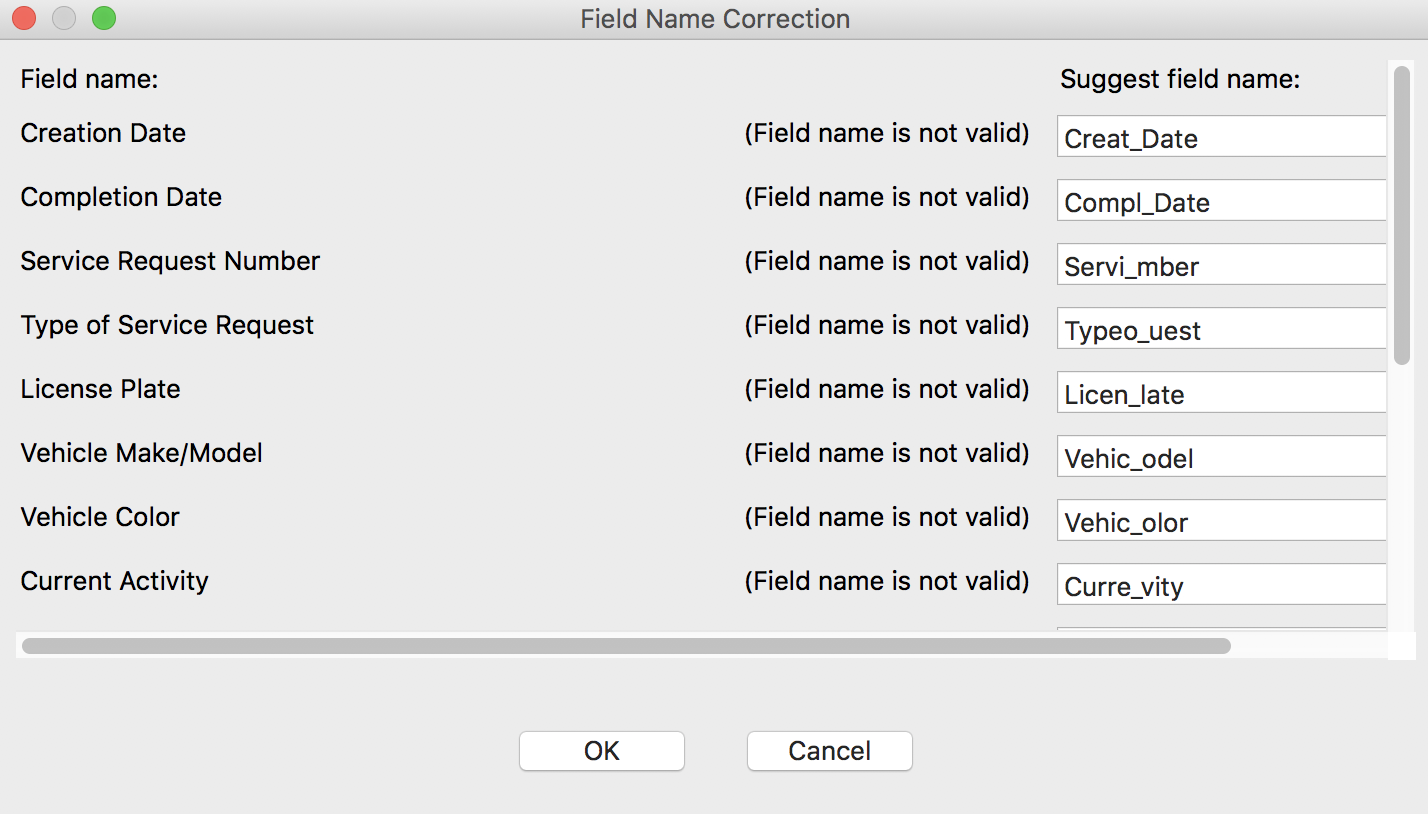
Variable Name Correction Suggestion
However, the suggested names are not always that useful. So, instead of taking the defaults, we enter new variable names as shown in the list below.
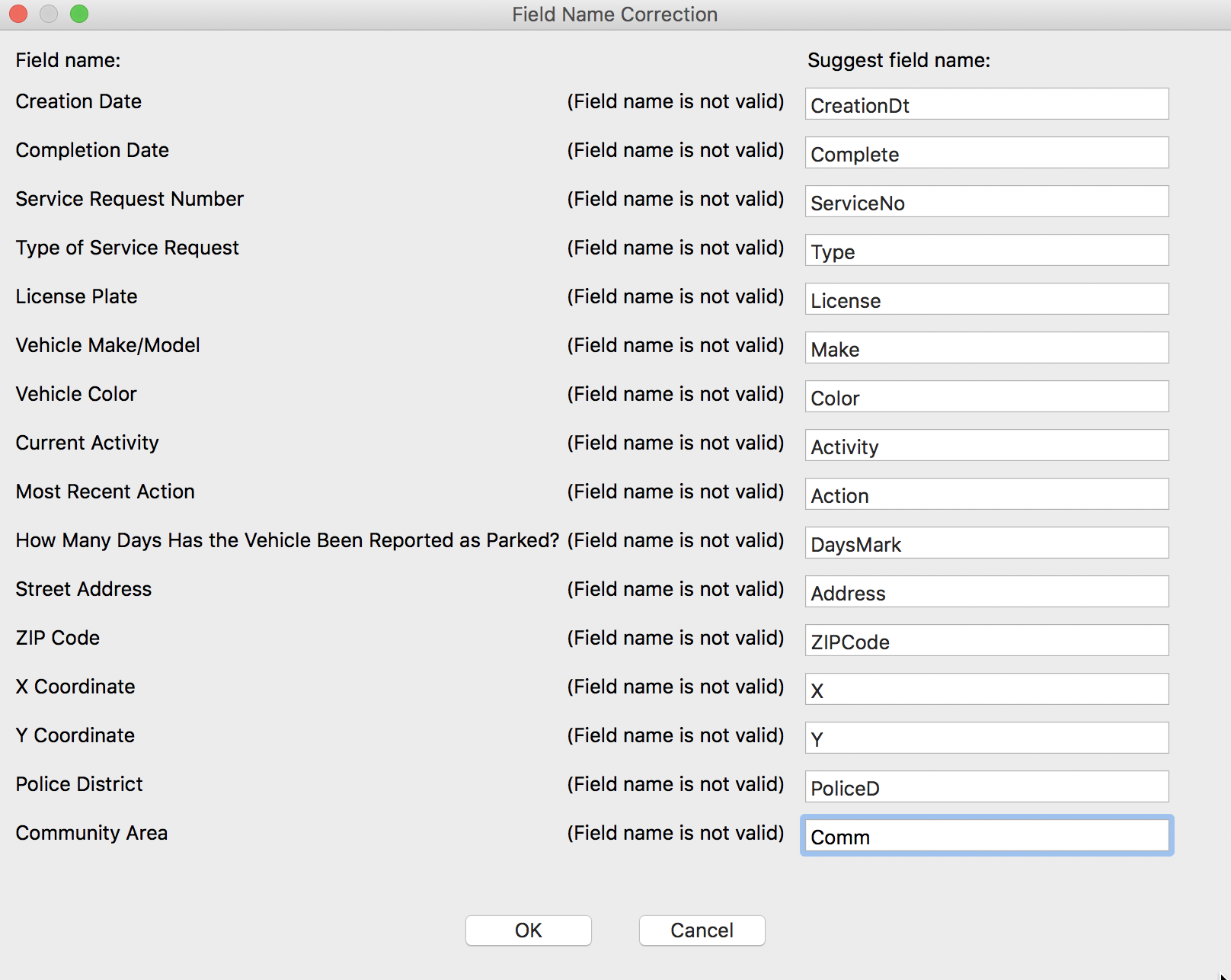
New Variable Names
Now, we can safely save the file.
We close the current project by selecting File > Close from the menu, or by selecting the Close icon from the toolbar (the second icon from the left).
Close Toolbar Icon
Make sure to reply that you do not want to save any changes. Don’t save the current project or the created geometries, you have already done that. Next, we start with a clean slate. At this point the Close icon should be dark (inactive).
We check the contents of the new file by selecting the Open icon and dragging the file vehicles.dbf into the Drop files here area. The table will open with the new content. The status bar reports that there are 2637 observations. The new variable names appear as the column headers.
New Data Table
More on selections
The feature of saving selected observations is used a lot in practice. It can be applied directly, as we have done here, but also indirectly. For example, sometimes we are interested in saving the table with the observations that do not meet a particular criterion. This is often the case when we have observations with missing values, or, in general, any observations we want to remove from the data set. First, we select those observations, but then we invert the selection, i.e., we take the complement. This can be done from within the Selection Tool, but also directly from the Table options menu, as Table > Invert Selection.
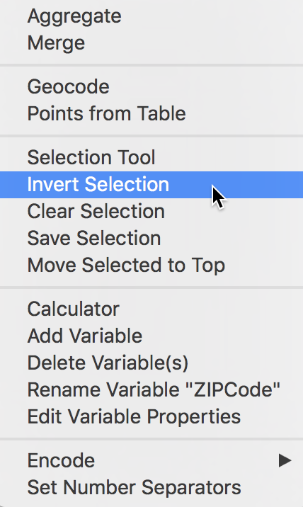
Invert Selection
If we now save the selected observations as a new file, this data set will no longer contain the observations we wanted to remove.
Another useful feature related to selections is the creation of an indicator (dummy) variable that typically takes the value of 1 for the selected observations and 0 for the others. Again, this can be accomplished both from within the Selection Tool as from the Table options menu, as Table > Save Selection. This should not be confused with File > Save Selection As. The latter creates a new file, the former adds a new variable to the current data set.
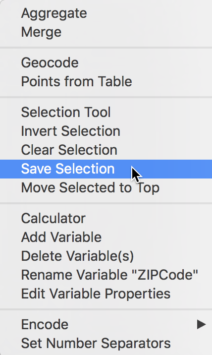
Save Selection
After choosing this option, a selection variable dialog appears that allows you to set a variable name (the default is SELECTED), as well as the values assigned to the selected and unselected observations. Typically, the default of 1 and 0 works fine, but there may be instances where other values might be appropriate (e.g., to flag particular observations with a specific code).
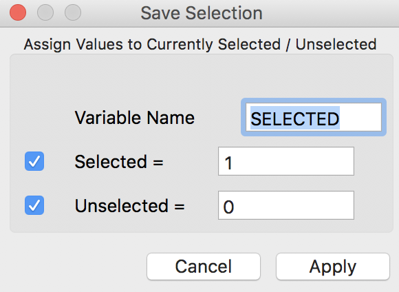
Selection Variable Dialog
Selecting the variables for the final table
The new table contains several variables that we are really not interested in. For example, both MONTH and YEAR have the same value for all entries, which is not very meaningful. Also, a number of the other variables are descriptive strings, that do not lend themselves to a quantitative analysis. As a final step, we will use the Table > Delete Variable(s) function (invoke from the menu or use right click in the table).
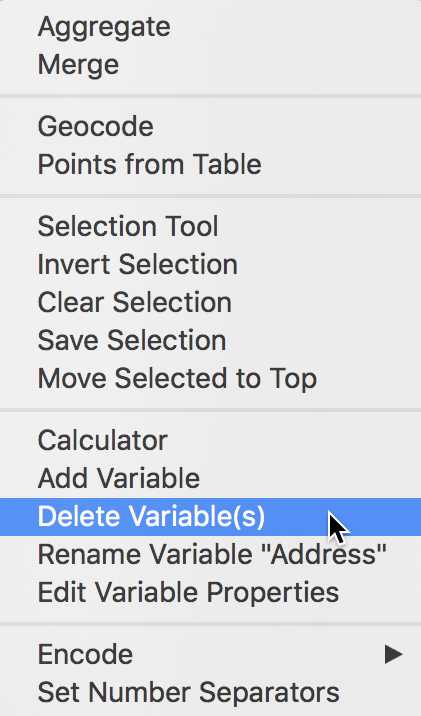
Delete Variables
The associated dialog lists all the variables in the current table. Select the variables to be deleted in the usual fashion, as shown below:
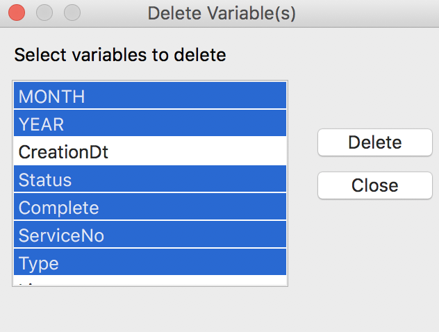
Delete Variables Dialog
In our example, we will only keep CreationDt, Address, ZipCode, X, Y, Ward, PoliceD, Comm, Latitude and Longitude. All the other variables should be selected in the dialog. Pressing the Delete button will remove them from the table. The final set of variable headings should correspond to the table below.
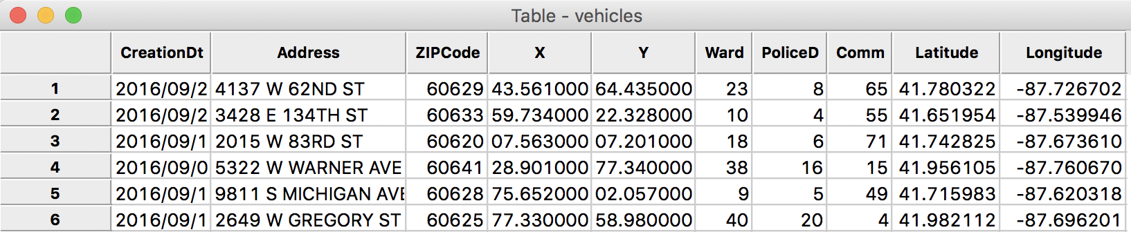
Final List of Variables
Finally, to make this change permanent, we Save the data by clicking on the save icon in the toolbar. This will replace the current vehicles.dbf file. To keep that file as a backup, we can instead use Save As with a new filename (in our example, we will overwrite the original file to keep things simple).
Save Toolbar Icon
Creating a Point Layer
So far, we have only dealt with a regular table, without taking advantage of any spatial features. However, the table contains fields with coordinates and GeoDa can turn these into an explicit spatial points layer that can be saved in a range of GIS formats. In the process of illustrating this, we will also tackle some typical data munging issues that result from data entry or other data quality problems. For example, in the current data set, there are two observations that have an entry of 0 for the community area. Since we will be aggregating the points by community area, it is critical that we have that information, or else we need to remove those observations. Luckily, in our case, there is a fairly straightforward solution, taking advantage of GeoDa’s spatial selection feature.
Creating a point layer from coordinates in a table
In GeoDa, it is straightforward to create a GIS point layer from tabular data that contain coordinate information. It is a two step process. After you invoke the function, a dialog appears to let you specify the X and Y coordinates. The Table > Points from Table item is one of the options in the Table menu.
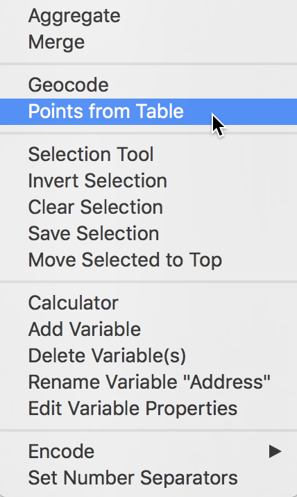
Points from Table (Table menu)
Alternatively, it can also be started from the main menu, as Tools > Shape > Points from Table.
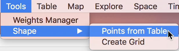
Points from Table (Tools menu)
In our example, the table contains two sets of coordinates, X and Y, as well as Longitude (the horizontal, or x-coordinate) and Latitude (the vertical, or y-coordinate). The X, Y variables are projected, and we will use those to illustrate a potential problem when no metadata on the projection is available.
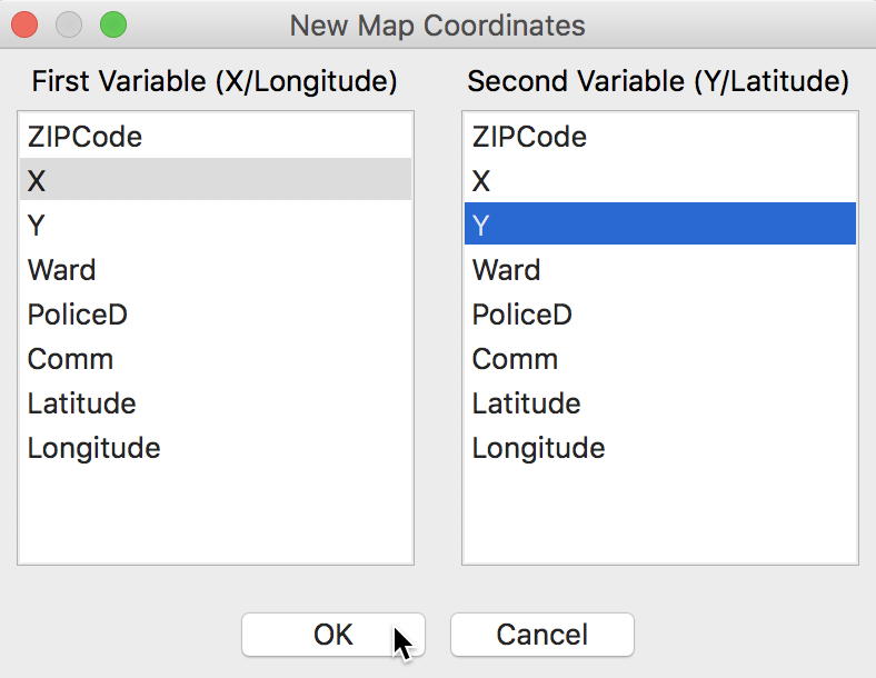
Specifying Coordinates
After clicking on OK, a warning message appears together with point map, showing the locations of the abandoned vehicles.
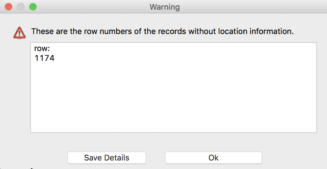
Missing Coordinates Warning
It turns out that one observation (in row 1174) does not have values for the X, Y coordinates. We will ignore this for now (we return to it below) and proceed to bring up the point map.2 When there are many observations with misbehaving coordinates, it may make sense to save the row numbers as a text file. This happens when clicking on the Save Details button. Instead, we will click OK and move on.
Note that the map legend and status bar mention 2636 observations, even though our table has 2637. This is another indication that one of the observations does not have a proper set of coordinates (which keeps them from being mapped).
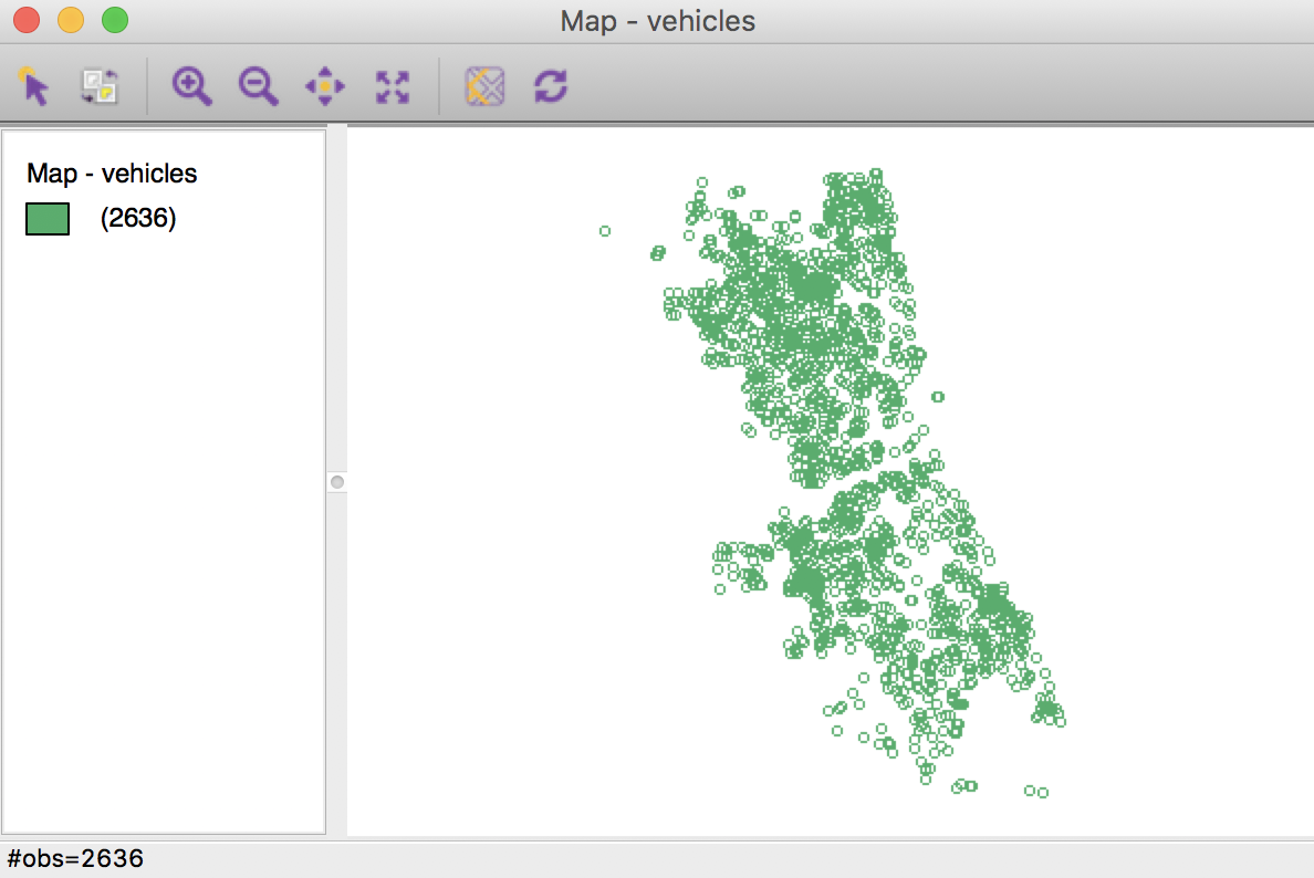
Point Map
To make this map into a GIS layer, we need to use Save As to convert it to one of the available formats. The save as file dialog (the small file folder icon) provides a list of the supported formats. We will use the ESRI shapefile format, and enter vehiclept for the file name.3
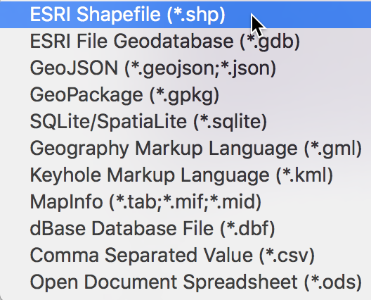
ESRI Shape File Format
Clicking on OK will create three files on the drive, with file extensions shp, shx, and dbf. The dbf file is the same as before, and contains the tabular data. The two other files contain information on the geometries. We can continue to work in the current project.
Data Problems
Gotcha #1 – missing projection information
The first problem we illustrate is the lack of metadata (data about data) on the projection. We can infer that the X and Y coordinates are projected from the units in which they are expressed. These are 7 digit values, likely corresponding to feet. But we don’t know what the projection is.
This becomes a problem when we try to combine these spatial data with other geographic information. For example, the map toolbar contains several special functions, represented by icons. The second from last brings up a Base Map, i.e., a background layer with realistic features, such as roads, rivers and lakes (similar to what you see in Google maps, Apple maps, etc.). This is not a real map in the GIS sense, but rather more like a background picture, but it often makes it easier to situate spatial features (like the points we created) in real space.
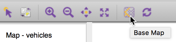
Base Map Icon
After selecting the Base Map option, a dialog appears with the various formats that are supported. For the sake of this example, we will pick Nokia Day.
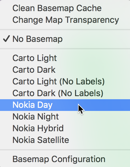
Base Map Format Options
But what happens? We do not get a base layer, but instead receive a warning message that the coordinate information is absent. This illustrates a very common problem that occurs when attempting to combine spatial data with incompatible projection information (in this case, missing information).
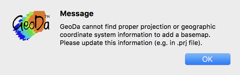
Projection Error Message
We will ignore this for now, since in what follows we will focus on the data in the table, without its explicity geometric features. We can proceed this way since our objective is to aggregate the points by community area, and we already have a community area code. In practice, this may not be the case, and you may need to carry out a spatial join in a GIS (which will require the projection information).
At this point, we can close the project – make sure to respond No to the query about saving the geometries, since we have already done that (in the vehiclept shape file).
Gotcha #2 – missing coordinates
With a clean project, we now load the just created shape file by dropping vehiclept.shp into the Drop files here box of the data connection dialog. Note that you only need to select the file with the shp extension, not all three files!
We get the same point map as when we created the points, but again with a warning message about the empty coordinates. In order to find out what is going on with the observation in question, we open the table by means of the Table icon on the main toolbar (the fourth item on the toolbar).
Table Toolbar Icon
In the table, we can sort the observations according to a given variable by double clicking on the corresponding field header. As an aside, this is an often used procedure to check for data problems, in the same spirit as computing the minimum and maximum. In our example, we are particularly interested in the coordinates, so we double click on X (or, alternatively, on Y). The small > indicates the sorted field and an ascending sorting order (low to high). Double clicking again reverses the sort order. To return back to the original order of observations, double click on the empty field header above the row numbers.
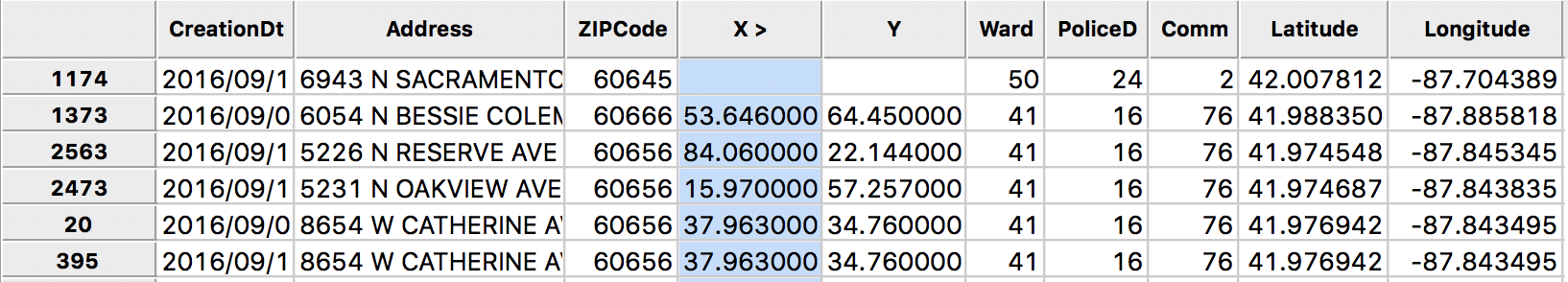
Missing Coordinates in Table
We see that indeed, observation 1174 does not have an entry for X or Y (interestingly, it does have an entry for Latitude and Longitude). However, there is an entry for the community area identifier, which is our main interest at this stage. Furthermore, since we won’t be using the actual point features, but only the information in the table, we can move on and ignore this issue.
Gotcha #3 – missing community area codes
There remains another problem, however. Moving back to the data table (click on the Table icon if necessary), we will now sort on the community area entries by double clicking on the Comm field header. As it turns out, the two smallest values are 0, which is an invalid code. Since we will be aggregating the points by community area, this if of concern.
We select the two observations with Comm = 0 by clicking on their row number on the left. Once selected, they will be highlighted in yellow, as shown in the table. They are also immediately selected in the corresponding point map, as shown by their stronger green color than the rest of the points (the points that are not selected become transparent).4 This illustrates the very important concept of linking. In GeoDa, a selection in any of the windows (for now, just the table, but later we will see that this extends to all graphical windows as well) is immediately also selected in all the open windows. In our example, this meant that the moment we selected the two observations in the table, they were also selected in the map. We will return to this important feature when we discuss visual analytics in more detail.
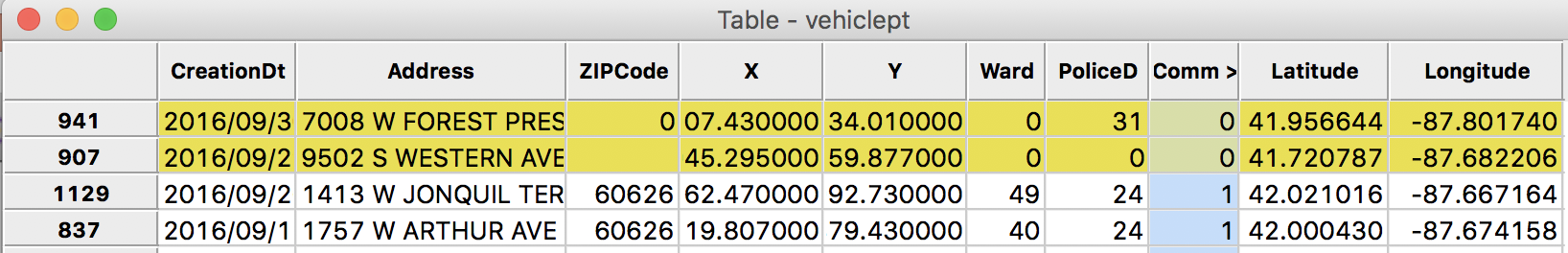
Sort Table by Community Area
How do we fix this? With a standard GIS, this is a point in polygon problem. We would combine the point locations with a layer of community areas and find the area in which the points are located. GeoDa does not have this functionality (yet). Instead, we can use an ad hoc approach that turns out to work well in this particular example. However, this is by no means necessarily always the case. Resorting to a point in polygon analysis is definitely best practice.
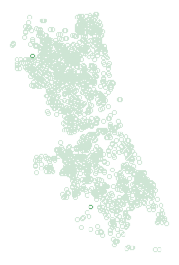
Selected Points in Map
We will now see if the values for neighboring points shed any light on which community area the two points in question may be located in. As long as the points are interior points to a community area (community areas are fairly large in Chicago), that is a reasonable approach.
We will invoke the Select icon of the map toolbar, the arrow sign that is the right-most icon.
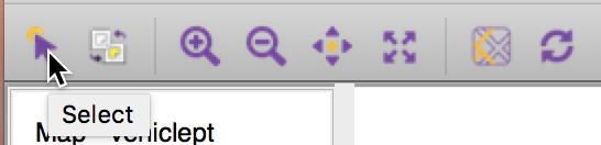
Map Selection Icon
This allows us to carry out a spatial selection, i.e., to click on a point or draw a rectangle (or circle) around it to select observations. This is a spatial counterpart to the various queries we used so far by means of the Table Selection Tool. When we draw a small rectangle around the point in question, the selected points keep their green color, but the other points become a much lighter shade of green. This is the way selected spatial items are shown in a map in GeoDa. We will return to the various spatial selection options when we discuss GeoDa’s mapping functionality in more detail in a later exercise.
We draw a small rectangle around the upper left point. The status bar shows how many observations are selected. In this example, around 10 is a good choice. When you select too many points, the odds of ending up in an ajoining community area go up.
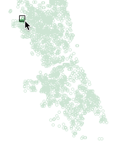
Select Point and Neighbors
In our example, we ended up with 11 points, but since this is a manual procedure, the results can differ a bit. The main idea is to keep the window small, and limited to the closest neighbors. The linking feature will result in the selected observations to be highlighted in the table.
To find out which observations were selected, we use the Move Selected to Top option in the table (either from the menu or by right clicking on the table).)
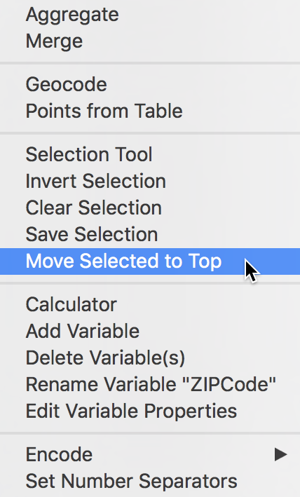
Move Selected to Top
This shows the observation contained in the selection window at the top of the table, highlighted in yellow. We see row 941 in the middle of the group with Comm as 0, surrounded by the other selected locations.
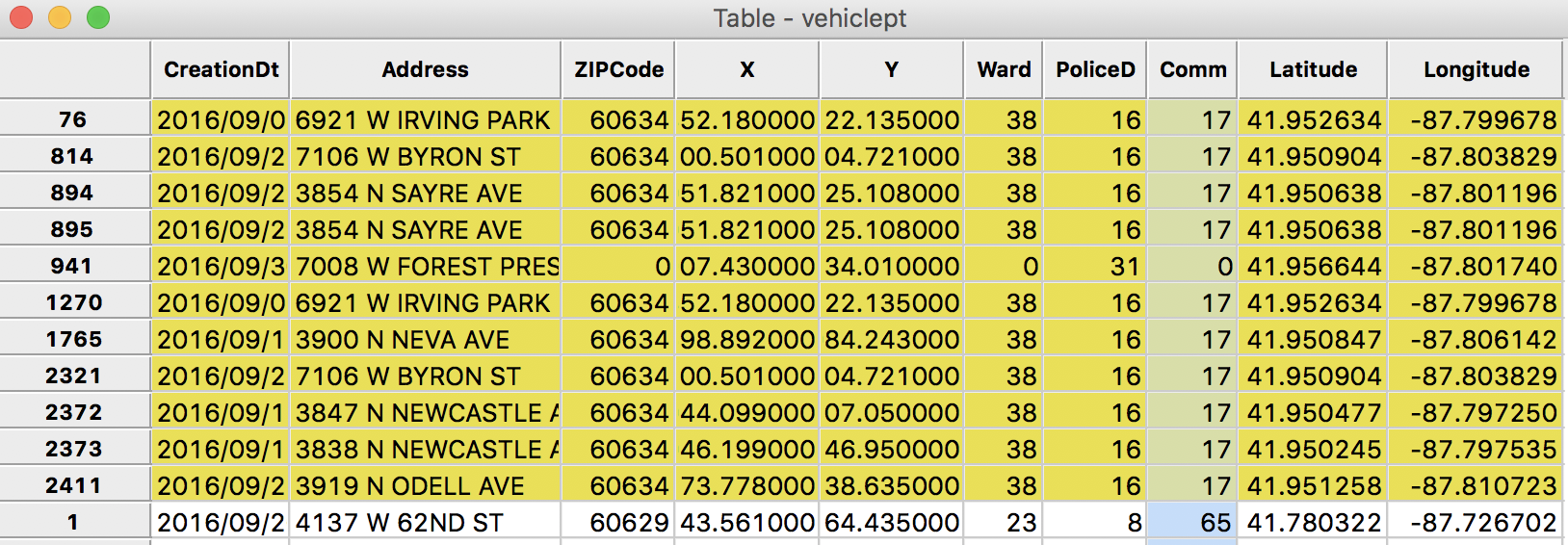
Selected Points in Table
In all likelihood, the missing value for the community area is 17, the same as for the 10 neighbors. We can now fix the entry in the table by using the cell editing functionality. First, we click on the cell in question to select it.
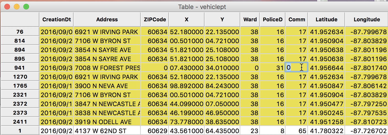
Edit Table Cell
Then, we enter the correct value (17) and press return to commit it to the table.
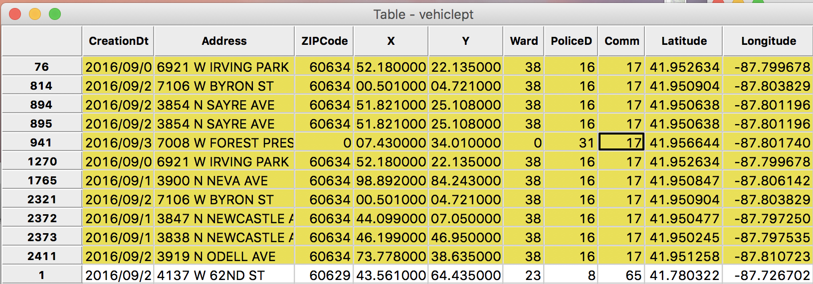
Table Cell Edited – 1
We now follow the same procedure for the other observation. For example, selecting four neighbors reveals that they are all in community area 72. So this is a likely entry, which we implement by means of the cell editing function. The result is as below.
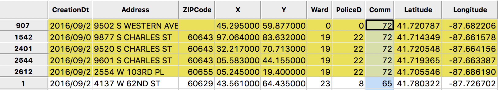
Table Cell Edited – 2
Finally, we can check the reverse order to see if the maximum value is correct, which gives 77 (77 is the number of community areas). At this point, we can save the new table (either Save to overwrite the current file, or Save As to create a new file). From now on, we will only use the data table by itself, as a dbf file, i.e., vehiclept.dbf.
Abandoned Vehicles by Community Area
Our ultimate goal is to map the abandoned vehicles by community area. But, so far, what we have are the individual locations of the vehicles. What we need is a count of the number of such vehicles by community area. In GIS-speak, this is referred to as spatial aggregation. The simplest case is the one we will illustrate here, where all we need is a count of the number of observations that fall within a given community area. Since we have the identifier for the enclosing community area for each of the individual vehicle locations, this is a simple table aggregation operation. In a GIS, the coordinates of the individual points would be subjected to a point in polygon operation, to determine the polygon (i.e., the community area) that encloses the point. In many situations in practice, the areal identifier will not be available, so that the only way to tackle this would be through an actual GIS operation.
The second case of aggregation is when the individual values of a variable are combined to a counterpart for the whole area. For example, if we wanted to count the total population in an area, and we have the number of people living in each house (represented as a point), we would want the sum of the population amounts, not just the count of observations in each area.
GeoDa support both types of aggregation operations, as long as a key is available, i.e., a unique identifier for the enclosing spatial unit. Specifically, in addition to the count of observations, GeoDa can compute the Average, Max, Min and Sum of the values for a variable over all the observations enclosed by the same areal unit.
To illustrate this feature, we start with a clean project, and load the dbf file with the vehicle locations that we just created, vehiclept.dbf, into GeoDa. Note that we only use the dbf file for this layer, and we ignore the shp and shx files. The reason for this is that there is nothing spatial about the aggregation operation as implemented, it is a simple row aggregation in a table.
The aggregation is invoked by selecting Table > Aggregate from the menu, or by right clicking to bring up the options menu in the table, in the usual way.
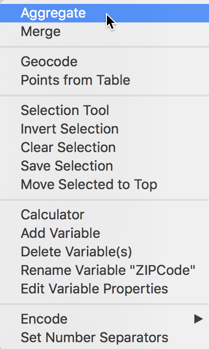
Table Aggregate
Selecting this option generates the Aggregate dialog. Here, we choose a radio button that corresponds with the operation we want. In our example, this is Count. We also need to specify the key, i.e., the unique identifier for each areal unit. Here, this is Comm for the community areas. For operations other than count, we would also have to select the variables to which the operation (e.g, sum, or max) will be applied. In our case, we do not need to do that. We click on the Aggregate button to bring up the familiar file saving dialog. Make sure to choose dBase Database File as the output format and set the file name to vehicle_count.dbf. A Success message will confirm that the new file was written to disk.
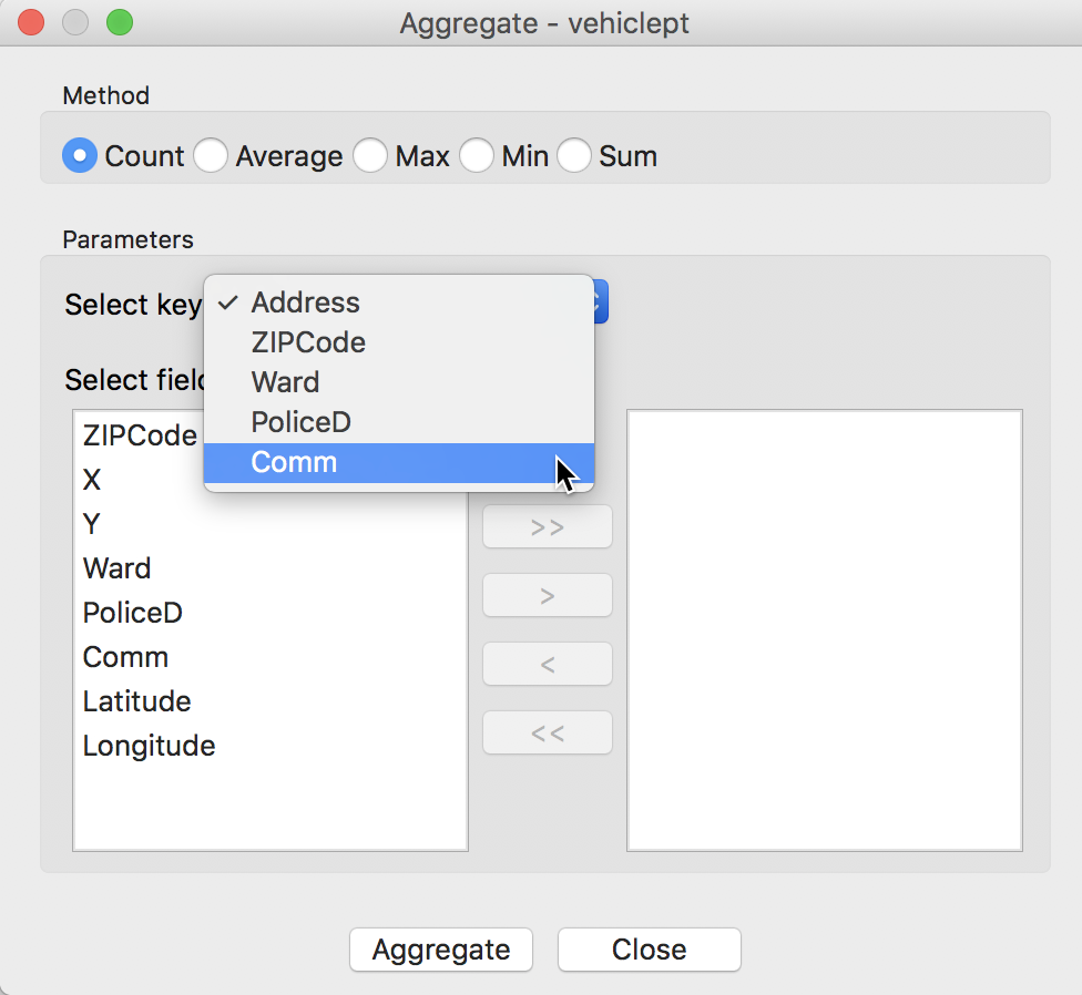
Select Aggregation Key
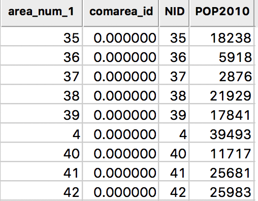
We can quickly check the contents of the file by closing the project and loading the new file. The table has two fields, one with the community area identifier, Comm, and one with the count of vehicles, AGG_COUNT.
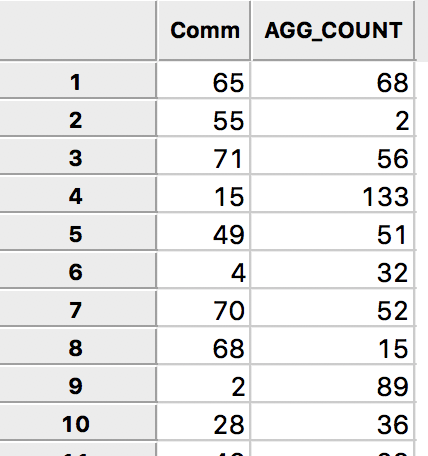
Vehicle Count by Community Area
We now have everything we need in terms of abandoned vehicle counts by community area, but we still need to specify the spatial data layer for the areas themselves.
Community Area Data
Since our ultimate objective is to create a choropleth map with the abandoned vehicles per capita for the Chicago community areas, we need two more pieces of information. We need a boundary file for the community areas so that we can create a base map, and we need the population data.
Community Area boundary file
Again, we resort to the City of Chicago open data portal for the boundary file. From the opening screen, select the button for Facilities & Geo Boundaries. This yields a list of different boundary files for a range of geographic areal units.
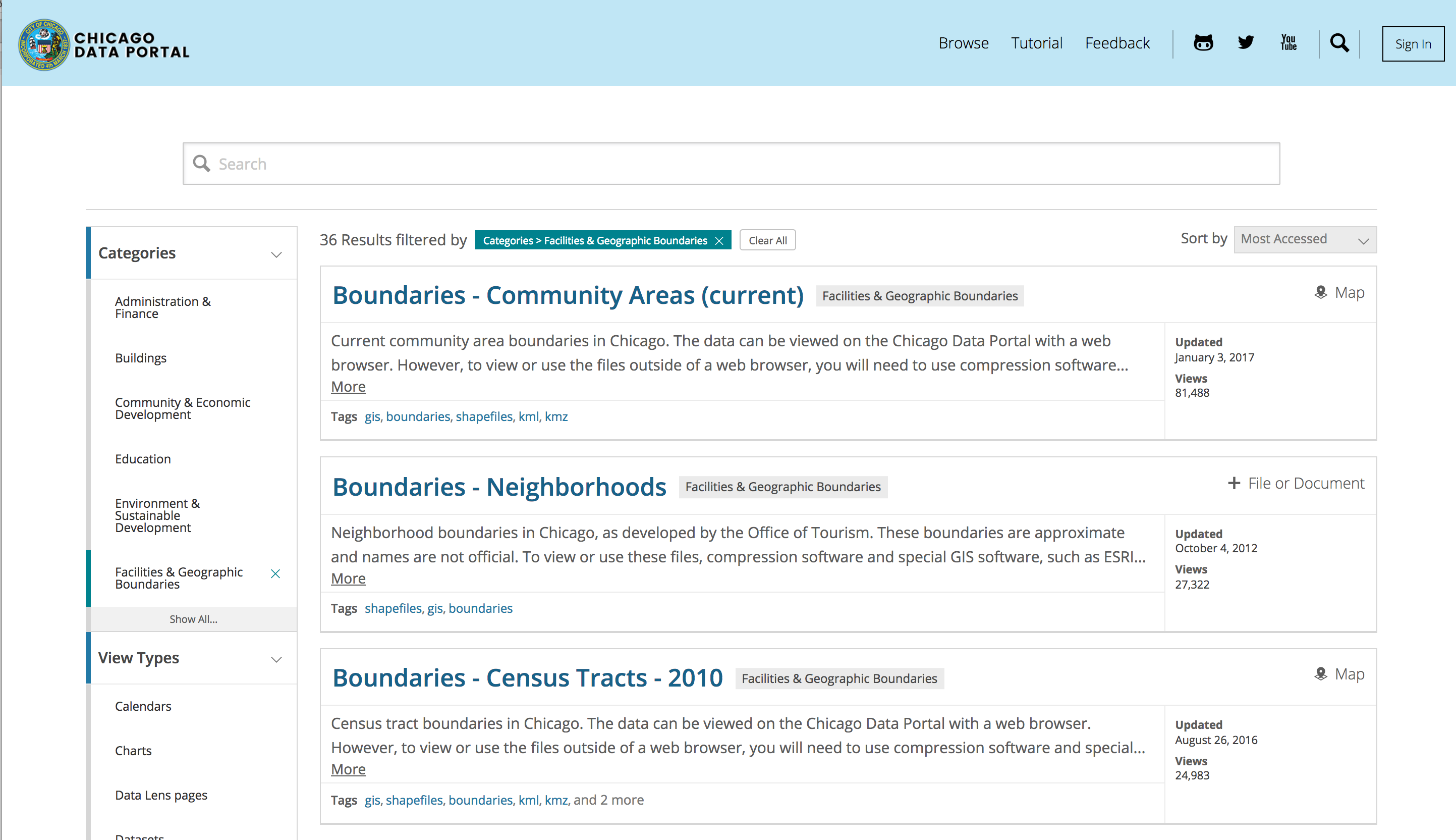
Chicago Boundary Files
We select Boundaries - Community Areas (current), which brings up an overview map of the geography of the community areas of Chicago:
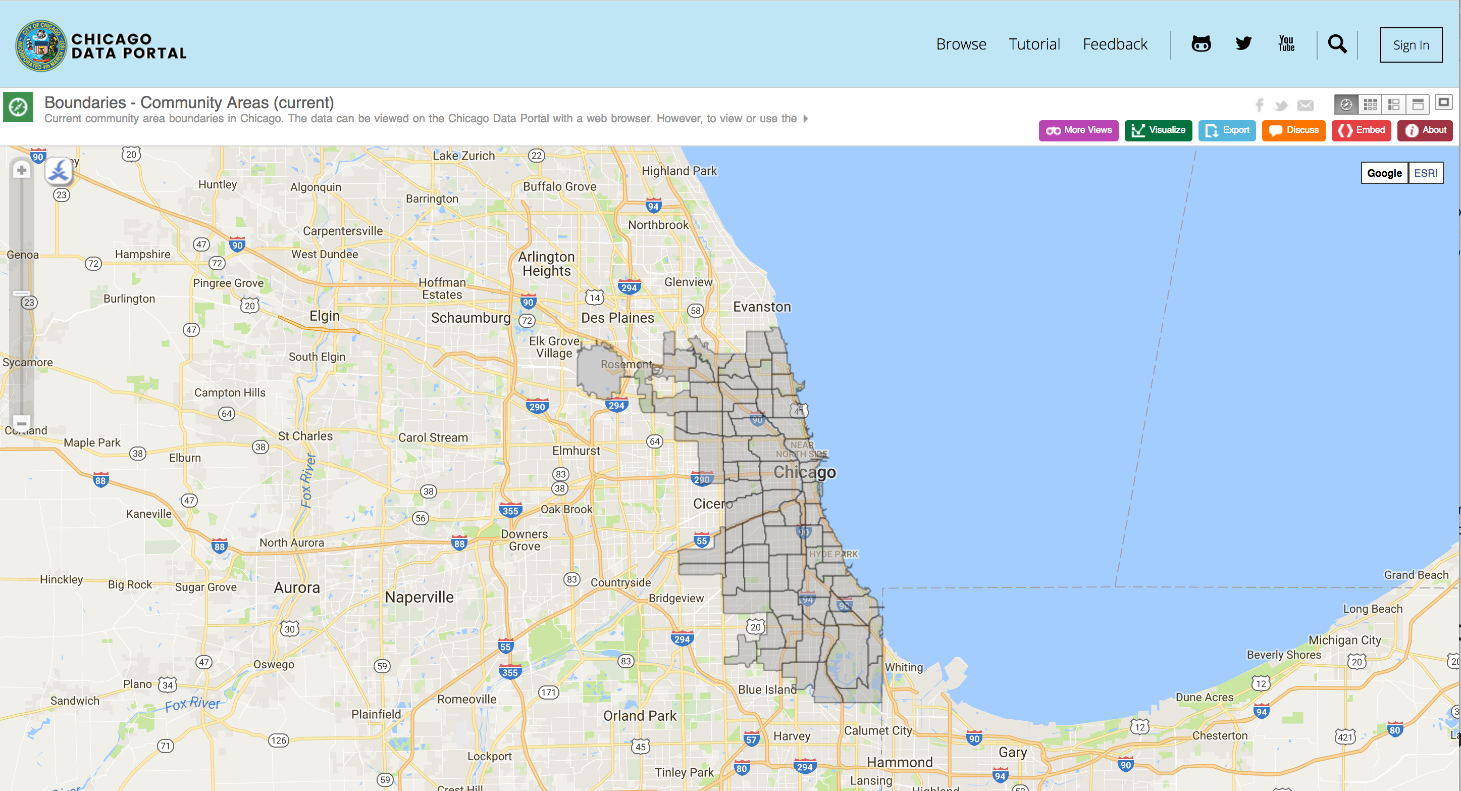
Chicago Community Areas
When we choose the blue Export button in the upper right hand side of the web page, a drop down list is produced with the different export formats supported by the site. We select Shapefile, the ESRI standard for boundary files.
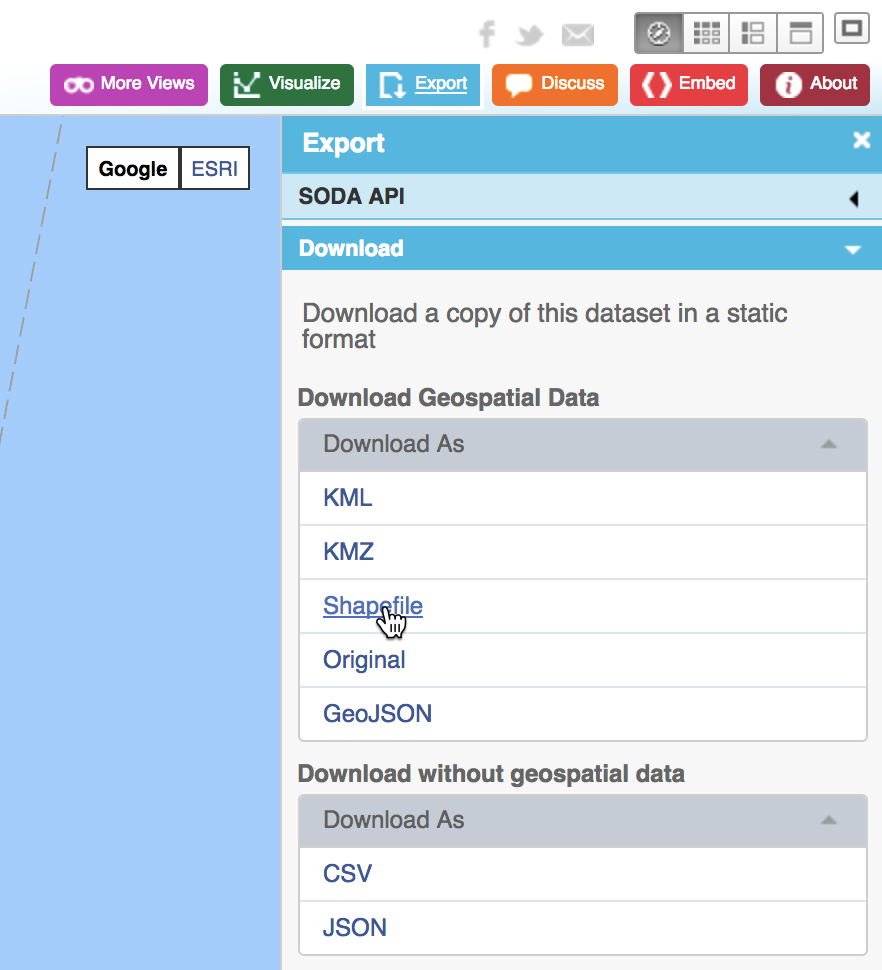
Download Boundaries as Shape File
This will download a zipped file to your drive that contains the four basic files associated with a shape file, with file extensions shp, shx, dbf and prj. The file name is the rather uninformative geo_export_fe02e535-53d6-4d62-a22b-7d06167b5a7c. For ease of interpretation, we change the four file names to chicagocomm.
Base map
To generate a base map for the community areas, we start a new project in GeoDa and drop the file chicagocomm.shp into the Drop files here area of the data source dialog. This will open a green base map, as shown below. Note how the status bar lists the number of observations (77).
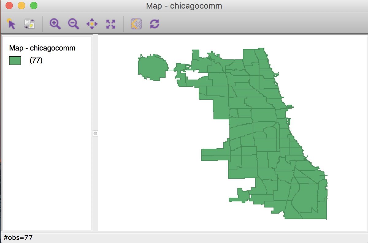
Community Area Base Map
We will return to the mapping functionality later. First, we check the contents of the data table by clicking on the Table icon in the toolbar. The familiar table appears, listing the variable names as the column headers and the contents for the first few observations.
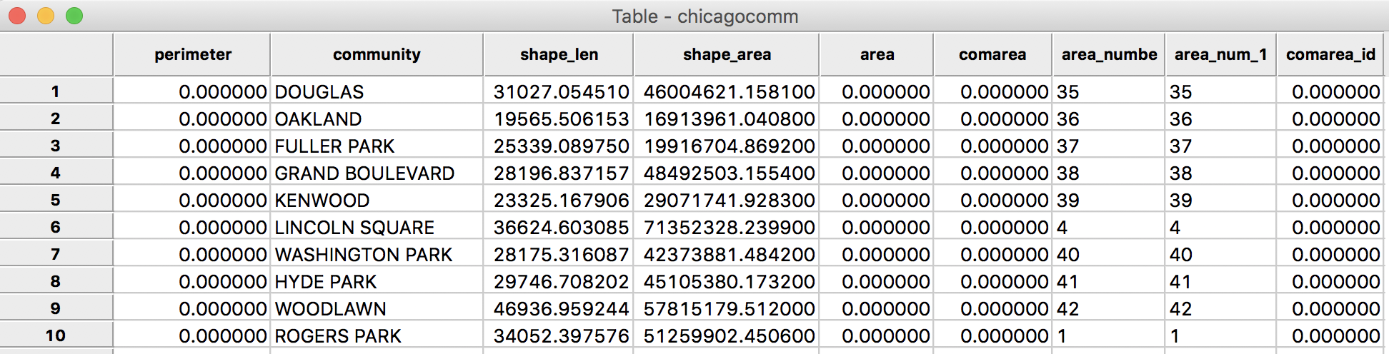
Community Areas Initial Table
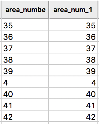
When we examine the contents closer, we see that we may have a problem. The values for area_numbe and area_num_1 (which are identical), corresponding to the Community Area identifier, are aligned to the left, suggesting they are string variables. For effective use in selecting and linking observations, they should be numeric, preferably integer.
We again use the Table > Edit Variable Properties functionality to change the variable format. We proceed as before, but now change the string format to integer. When invoking the function, the type for area_num_1 shows string. We click on this value and change it to integer.
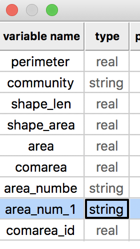
String to Integer Format Conversion
After the conversion, we will see the values for area_num_1 right aligned in the table, as numeric values should be.
Community ID as Integer
To make this change permanent, we again Save the data by clicking on the save icon in the toolbar (no need to Save As since we don’t really want to keep the ID variable as a string).
A note on projections
A detailed treatment of projections is beyond the scope of our discussion, but it is nevertheless a critical concept. The bottom line is that whenever two geographical layers are to be combined, they need to be expressed in the same projection. This is a (very) common source of problems when integrating different spatial data sets. A projection consists of two important pieces of information. One is the model for the earth spheroid (the earth is not a ball, but a sort of ellipsoid), and the second is the transformation used to convert latitude and longitude degrees to cartesian coordinates (Y for latitude and X for longitude). For ESRI shape files, this information is contained in the file with the .prj extension. More generally, this is a file with the coordinate reference system (or CRS) information in it. There are a number of formats. A good resource is the spatialreference.org site, which contains thousands of references in a variety of commonly used formats.
For our purposes, we will just need to make sure that whenever we join or merge two spatial data sets, they both have the same .prj file. More complex manipulations will require a full-fledged GIS system, or the use of the proj4 library in R. See also the tutorial on spatial data analysis and visualization in R by Guy Lansley and James Cheshire for an excellent overview of the main issues with examples using R.
Community Area population data
In order to compute the number of abandoned vehicles per capita, we need some population values for the community areas. As it turns out, it is not that simple to find this in a readily available digital format. The City of Chicago web site contains a pdf file with the neighborhood ID, the neighborhood name, the populations for 2010 and 2000, the difference between the two years and the percentage difference. While pdf files are fine for reporting results, they are not ideal to input into any data analysis software. Since there are only 77 community areas, we could sit down and just type the values, but that is asking for trouble. Instead we should use a data scraping tool, such as the functionality contained in the R package pdftools. To save some trouble, the results of this operation with population data for 2010 are included in the file Community_Pop.csv.
Merging the population data
We start with having the Chicago Community area base map active, with the table open. Right click on the table, or use the menu to select Table > Merge, as shown:
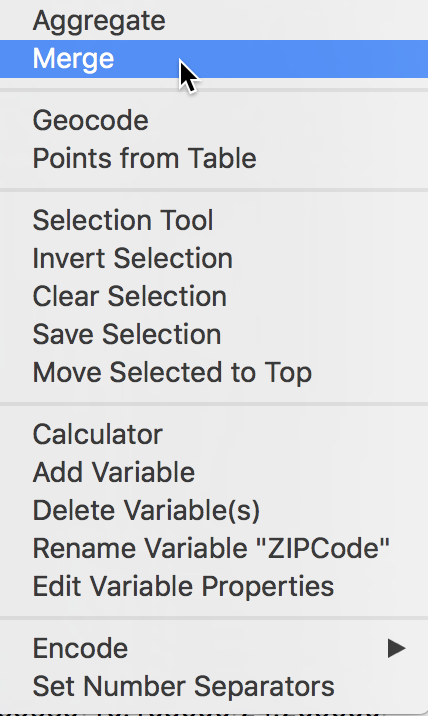
Table Merge
This brings up a dialog to select the data source to be merged. GeoDa can read and write a range of formats, as we have already seen when saving the CSV file as a DBF. Click on the file folder icon associated with the Select datasource box to bring up the data source selection dialog. As before, drop the file Community_Pop.csv into the Drop files here area. This will populate the Merge dialog with candidate key variable names as well as the variables present in the data set to be merged. The radio button for Merge is selected. The difference between the two options is that Stack is to add observations to an existing data set (and given set of variables), whereas Merge is to add variables to a current set of observations. The second radio button is to Merge by key values. This is the preferred approach, since it matches observations between the two data sets on identical values (integer) for a key variable. The name for the key variables do not need to be the same, but the values must match. It is also the standard approach taken when implementing a join in a data base operation. The alternative is to Merge by record order which is only appropriate when there is absolute certainty that the two tables have the observations in exactly the same order.
In our example, the datasource is Community_Pop, and the current table key should be set to area_num_1 (which we just turned into an integer field), with the import table key as NID (also an integer). Note that the initial default of community for the current table key is not appropriate. Before selecting the variables to be merged in, the dialog should be as below:
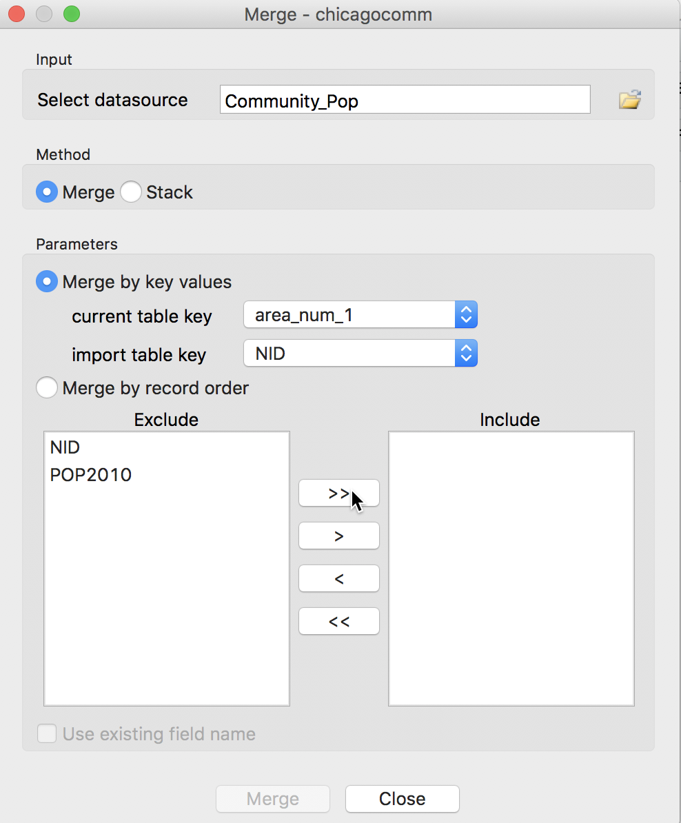
Table Merge Variable Selection Dialog – 1
Since we want all the variables merged in (it is always a good idea to keep the matching key to make sure everything works as advertised), we use the double arrow button >> to move all the variables from the Exclude to the Include panel. If only selected variables need to be merged in, we can use the single arrow button > to select them individually. The reverse arrows move variables back into the Exclude panel.
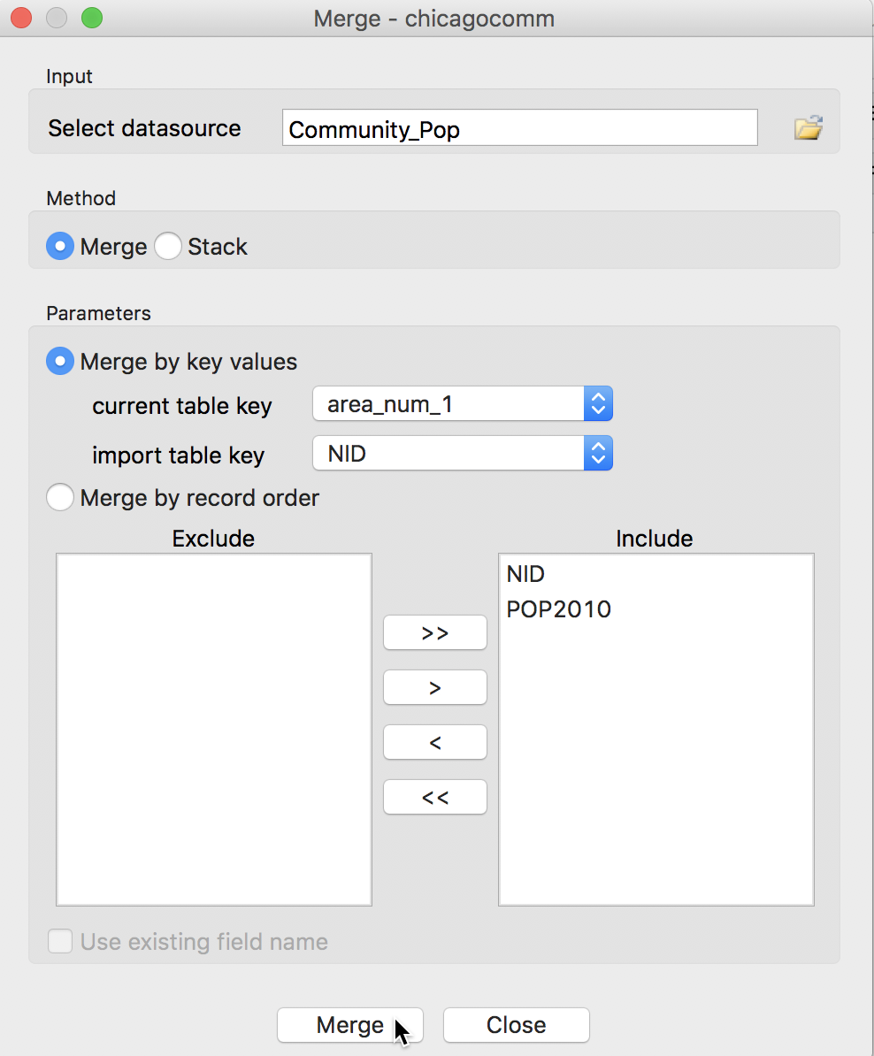
Table Merge Variable Selection Dialog – 2
To execute the merge operation, we click on the Merge button. If successful, a brief message to that effect will appear. If not, there will be some indication of what may have gone wrong. Typically, this can be due a mismatch in the key variables or the non-uniqueness of the values for a key variable. In our example, after proceeding with the merge, we see the two new variables NID and POP2010 added as additional columns at the end of the table.
Variables after Merge
Finally, we do some cleanup and use the Table > Delete operator to eliminate all the variables we are not interested in. In the end, we keep only the four variables community, area_num_1, NID and POP2010, as shown below.
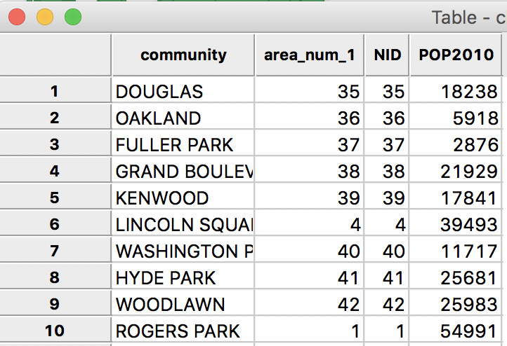
Cleaned up Table
We make the changes permanent by clicking on the Save icon in the toolbar. The updated shape file chicagocomm now only includes the four variables we selected. At this point, we could use the Map functionality to create a choropleth map of total population. However, this is not advisable, since total population is a so-called spatially extensive variable, in the sense that it will tend to be larger for larger areas, everything else being the same. In other words, the larger population size may be only related to an area being larger and not to any other underlying process. In general, it is good to avoid mapping spatially extensive variables and replace them by spatially intensive counterparts, such as a population density. We take this approach and do not map the total counts for the abandoned vehicles, but turn it into a per capita ratio instead.
Mapping Community Area Abandoned Vehicles Per Capita
At this point, we have all the pieces to proceed with our final map. There are three tasks remaining: merge the vehicle counts table with the community area layer; compute the per capita rate; and create a choropleth map.
Merging the vehicle count table with the community area layer
To merge the vehicle count table with the community area layer, we proceed in the same fashion as before. We start by loading the chicagocomm.shp file onto the Drop files here area, and use the Table icon to open the associated table. In the menu (or, by right clicking in the table), we select Table > Merge. We select the datasource to be merged in as vehicle_count.dbf (this is the table we created by aggregating the abandoned vehicle events by community area). The matching keys are area_num_1 in the community area layer and Comm for the vehicle counts. We move both variables in the vehicle count data set to the Include panel. Before merging, the dialog should look as shown below.
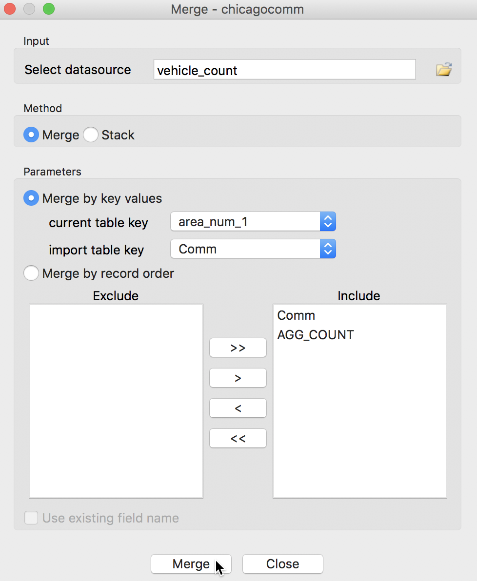
Merge Table Dialog for Vehicle Counts
After clicking on the Merge button, two new columns are added to the community area layer. In the new table, we now have both the population (POP2010) and the count (AGG_COUNT).
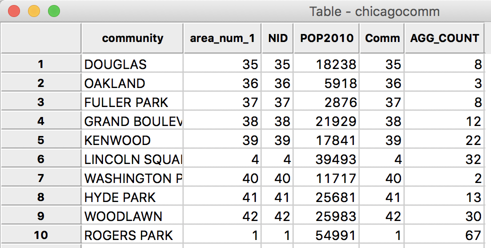
Vehicle Counts Merged
We make the change permantent by pressing the Save button, or, alternatively, Save As under a different file name, although at this point, this is not necessary, since we are proceeding immediately to the rate computation.
Computing abandoned vehicles per capita
The number of vehicles per capital is computed by means of the by now familiar Calculator tool. We first Add a new variable, e.g., VEHPCAP (place the field after the last variable) and then use the Bivariate tab to calculate the division (DIVIDE) of AGG_COUNT by POP2010, as shown below.
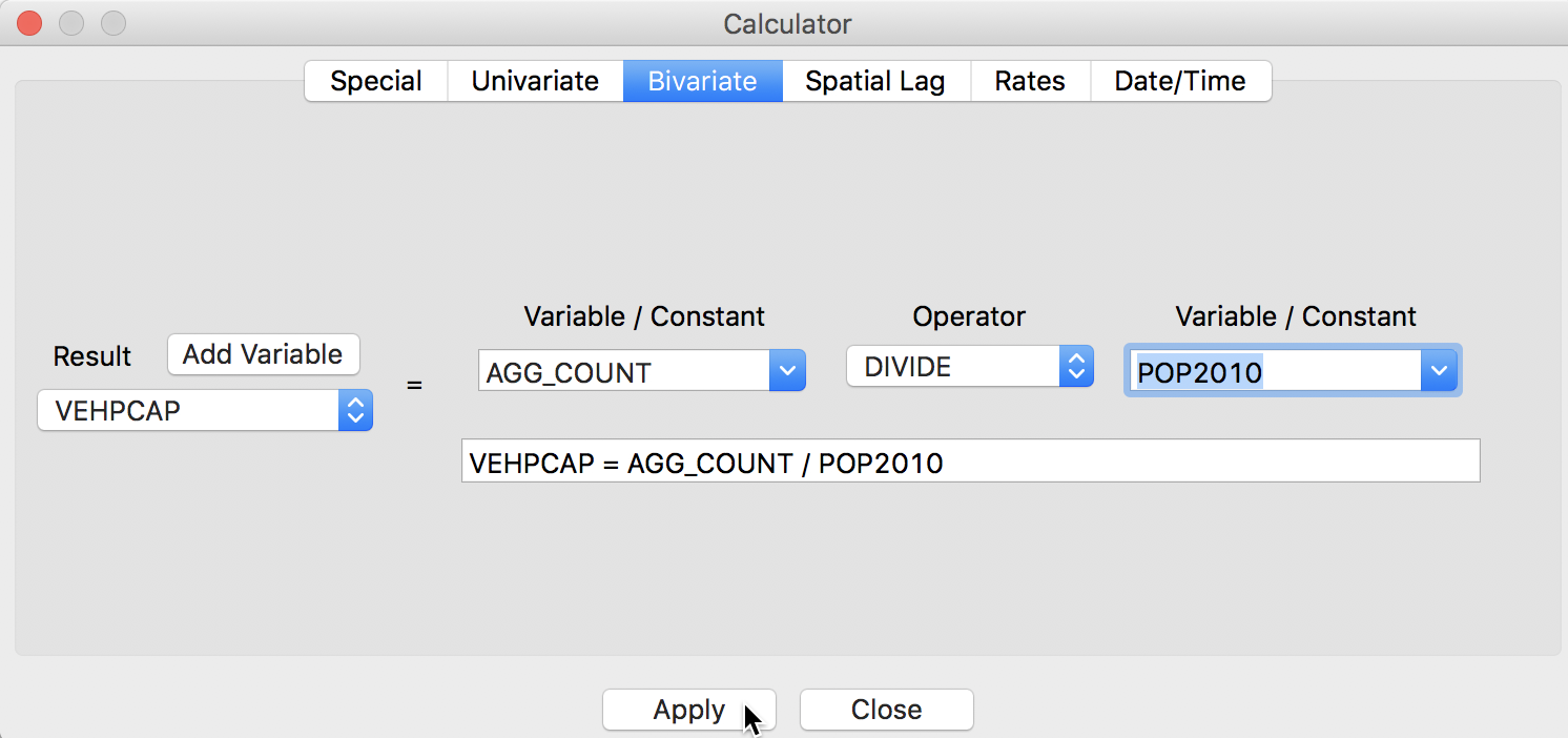
Compute Per Capita Abandoned Vehicles
The resulting values are very small and not that easy to interpret. So, we use the Calculator again to compute the abandoned vehicles per 1000 population. The new variable VHC1000 is simply VEHPCAP multiplied by the constant 1000 (use the Bivariate tab, with MULTIPLY, VEHPCAP in the first and the constant 1000 entered in the second Variable/Constant box). The final data table consists of eight columns, as shown.
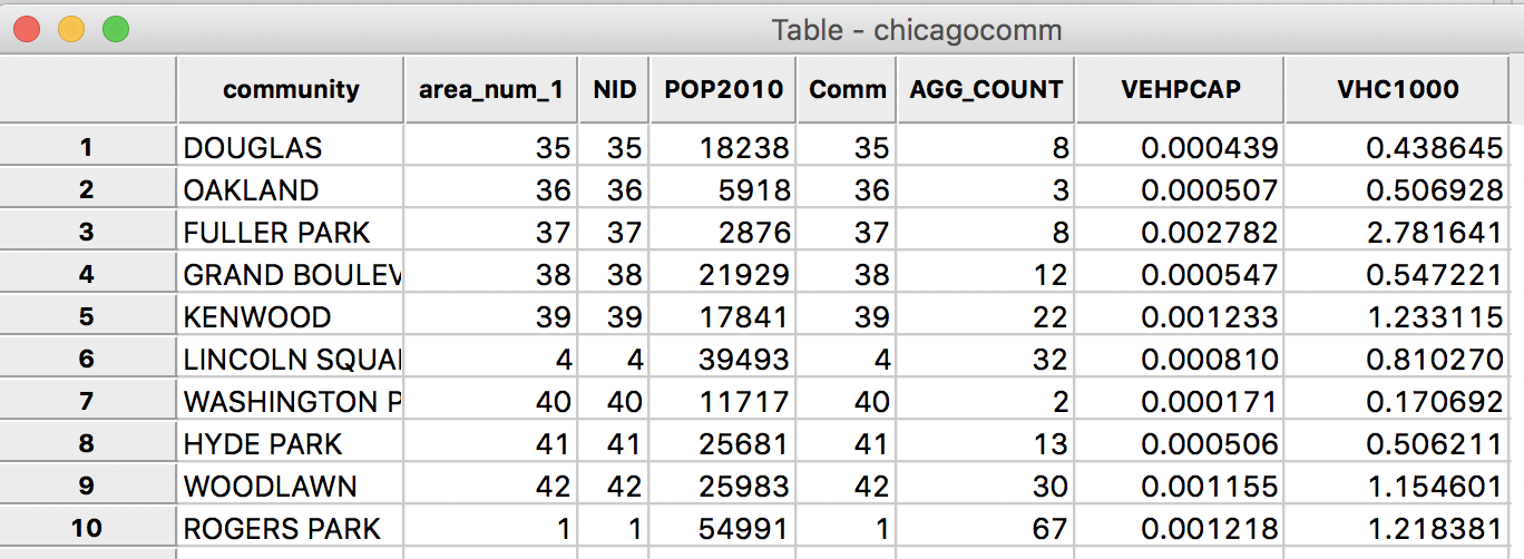
Final Set of Variables
At this point, we may want to make the changes permanent, with either the Save or Save As operations.
Choropleth map
We now move beyond the Table functionality in GeoDa and proceed to create a map. This is initiated either from the menu or by clicking on the Map toolbar icon (the sixth icon from the left on the toolbar).
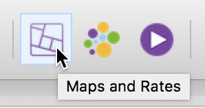
Map Toolbar Icon
This brings up the menu of map options (the same as when selecting Map from the main menu). We will keep things simple (we explore mapping in much more detail in a later excercise) and create a quintile map, i.e., a quantile map with 5 categories (each quintile corresponds to 20% of the observations, sorted in ascending order). We select Quantile Map from the list and click on 5 for a quintile map.
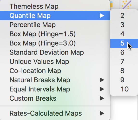
Quintile Map Option
The following dialog asks for the variable to be mapped. We choose VHC1000 for the number of abandoned vehicles per 1000 population.
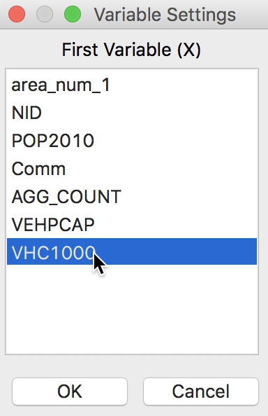
Map Variable Selection
After clicking on the OK button, the quintile map appears. Because 77 (the number of observations) does not divide cleanly into 5, three categories have 15 observations and two have 16 (in a perfect quintile world, they each should have exactly the same number of observations). The number of observations is given within parentheses in the legend. The intervals for each of the 5 categories are given in the legend as well.
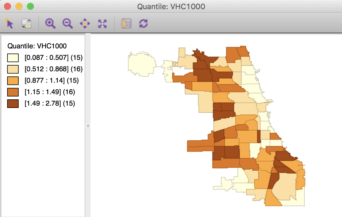
Quintile Map – Abandoned Vehicles
As before, we can add a base layer to this map to reflect the on the ground geography of Chicago. We click on the second icon from right in the map toolbar (the Base Map icon) and choose Nokia Day from the drop down list. In contrast to our frustrating experience earlier, the base layer appears. This is because we have proper projection information for the community area layer (remember the prj file!).
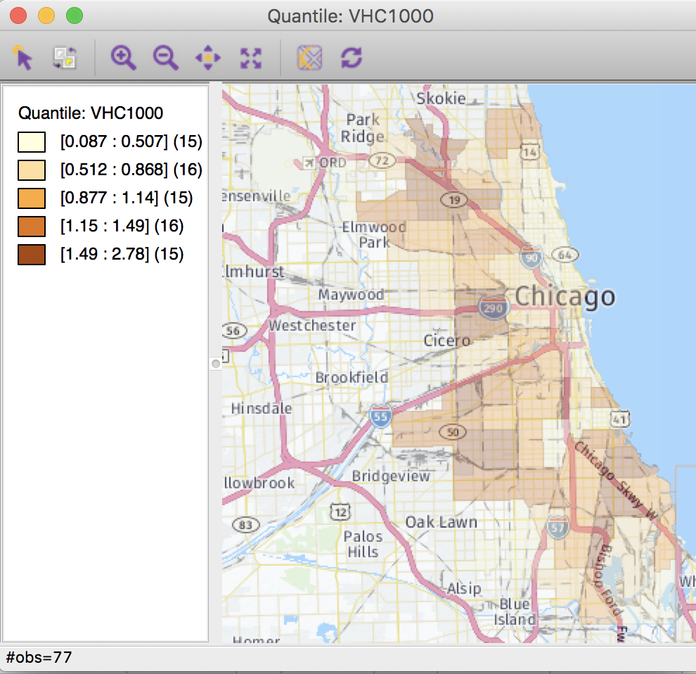
Abandoned Vehicles with Base Map
We can adjust the relative transparency between the two layers (Change Map Transparency in the drop down menu associated with the Base Map icon), but we will leave matters as they are for now.
This ends our journey from the open data portal all the way to a visual representation of the spatial distribution of abandoned vehicles. The maps do suggest some patterning and some potential association with proximity to the major interstates, but we will leave a more formal analysis of patterns (and clusters) to a later exercise.
References
Dasu, Tamraparni, and Theodore Johnson. 2003. Exploratory Data Mining and Data Cleaning. Hoboken, NJ: John Wiley & Sons.
-
University of Chicago, Center for Spatial Data Science – anselin@uchicago.edu↩
-
In earlier versions of GeoDa, the empty coordinates would be interpreted as 0,0 and included on the point map. Typically, this would result in an extreme point in one of the lower corners, and a miniature view of Chicago in the opposite corner. As of Version 1.12 of GeoDa, the empty coordinates are ignored and a map is produced for all the valid points.↩
-
The term shape file is a bit of a misnomer, since it is not a single file, but a collection of files, all with the same name, but with different file extensions.↩
-
There are other ways to highlight selections in GeoDa, as detailed in the Preferences.↩