3 Buffer Analysis
3.1 Overview
Once we have spatially referenced resource locations, it’s helpful to plot the data in the community of interest for some preliminary analysis. In this tutorial we will plot Methadone Providers in Chicago and community areas to provide some context. We will also generate a simple 1-mile buffer service area around each provider to highlight neighborhoods with better, and worse, access to resources. In order to accomplish this task, we will need to standardize our spatial data (clinic points, and community areas) with an appropriate coordinate reference system. Finally, we’ll make some maps!
Our objectives are thus to:
- Overlay clinical providers (points) and community areas (polygons)
- Use a spatial transform operation to change coordinate reference systems
- Conduct a simple buffer analysis
3.2 Environment Setup
To replicate the code & functions illustrated in this tutorial, you’ll need to have R and RStudio downloaded and installed on your system. This tutorial assumes some familiarity with the R programming language.
3.2.1 Input/Output
Our inputs will be two shapefiles, and a geojson (all spatial file formats). These files can be found here, though the providers point file was generated in the Geocoding tutorial. Note that all four files are required (.dbf, .prj, .shp, and .shx) to consitute a shapefile.
- Chicago Methadone Clinics,
methadone_clinics.shp - Chicago Zip Codes,
chicago_zips.shp - Chicago City Boundary,
boundaries_chicago.geojson
We will generate a 1-mile buffer around each point, and generate maps with the zip code areas for context. We will also export the final buffer areas as another shapefile for future use. Finally, we’ll generate a more beautiful map by including the city boundary.
If you don’t have a shapefile of your data, but already have geographic coordinates as two columns in your CSV file, you can still use this tutorial. A reminder of how to transform your CSV with coordinates into a spatial data frame in R can be found here.
3.2.2 Load Libraries
We will use the following packages in this tutorial:
sf: to manipulate spatial datatmap: to visualize and create maps
First, load the required libraries.
3.2.3 Load Data
Load in the MOUD resources shapefile.
## Reading layer `methadone_clinics' from data source `/Users/yashbansal/Desktop/CSDS_RA/opioid-environment-toolkit/data/methadone_clinics.shp' using driver `ESRI Shapefile'
## Simple feature collection with 27 features and 8 fields
## geometry type:  POINT
## dimension:      XY
## bbox:           xmin: -87.7349 ymin: 41.68698 xmax: -87.57673 ymax: 41.96475
## geographic CRS: WGS 84
Next, we load a shapefile of Chicago zip codes. You can often find shapefiles (or spatial data formats like geojson) on city data portals for direct download. We will walk you through downloading zip code boundaries directly through the Census via R in a later tutorial.
## Reading layer `chicago_zips' from data source `/Users/yashbansal/Desktop/CSDS_RA/opioid-environment-toolkit/data/chicago_zips.shp' using driver `ESRI Shapefile'
## Simple feature collection with 85 features and 9 fields
## geometry type:  MULTIPOLYGON
## dimension:      XY
## bbox:           xmin: -88.06058 ymin: 41.58152 xmax: -87.52366 ymax: 42.06504
## geographic CRS: WGS 84## Reading layer `boundaries_chicago' from data source `/Users/yashbansal/Desktop/CSDS_RA/opioid-environment-toolkit/data/boundaries_chicago.geojson' using driver `GeoJSON'
## Simple feature collection with 1 feature and 4 fields
## geometry type: MULTIPOLYGON
## dimension: XY
## bbox: xmin: -87.94011 ymin: 41.64454 xmax: -87.52414 ymax: 42.02304
## geographic CRS: WGS 84Quickly view the first few rows of the zip codes and clinics using your favorite function (head, glimpse, str, and so forth).
## Simple feature collection with 6 features and 9 fields
## geometry type:  MULTIPOLYGON
## dimension:      XY
## bbox:           xmin: -88.06058 ymin: 41.73452 xmax: -87.58209 ymax: 42.04052
## geographic CRS: WGS 84
##   ZCTA5CE10 GEOID10 CLASSFP10 MTFCC10 FUNCSTAT10  ALAND10
## 1     60501   60501        B5   G6350          S 12532295
## 2     60007   60007        B5   G6350          S 36493383
## 3     60651   60651        B5   G6350          S  9052862
## 4     60652   60652        B5   G6350          S 12987857
## 5     60653   60653        B5   G6350          S  6041418
## 6     60654   60654        B5   G6350          S  1464813
##   AWATER10  INTPTLAT10   INTPTLON10
## 1   974360 +41.7802209 -087.8232440
## 2   917560 +42.0086000 -087.9973398
## 3        0 +41.9020934 -087.7408565
## 4        0 +41.7479319 -087.7147951
## 5  1696670 +41.8199645 -087.6059654
## 6   113471 +41.8918225 -087.6383036
##                         geometry
## 1 MULTIPOLYGON (((-87.86289 4...
## 2 MULTIPOLYGON (((-88.06058 4...
## 3 MULTIPOLYGON (((-87.77559 4...
## 4 MULTIPOLYGON (((-87.74205 4...
## 5 MULTIPOLYGON (((-87.62623 4...
## 6 MULTIPOLYGON (((-87.64775 4...
3.3 Simple Overlay Map
We can plot these quickly using the tmap library to ensure they are overlaying correctly. If they are, our coordinate systems are working correctly.
When using tmap the first parameter references the spatial file we’d like to map (tm_shape), and the next parameter(s) indicate how we want to style the data. For polygons, we can style tm_borders to have a slightly transparent boundary. For the point data, we will use red dots that are sized appropriately using the tm_dots parameter. When working with tmap or any other library for the first time, it’s helpful to review the documentation and related tutorials for more tips on usability.
We use the tmap “plot” view mode to view the data in a static format.
## tmap mode set to plotting## 1st layer (gets plotted first)
tm_shape(areas) + tm_borders(alpha = 0.4) +
## 2nd layer (overlay)
tm_shape(metClinics) + tm_dots(size = 0.4, col="red") 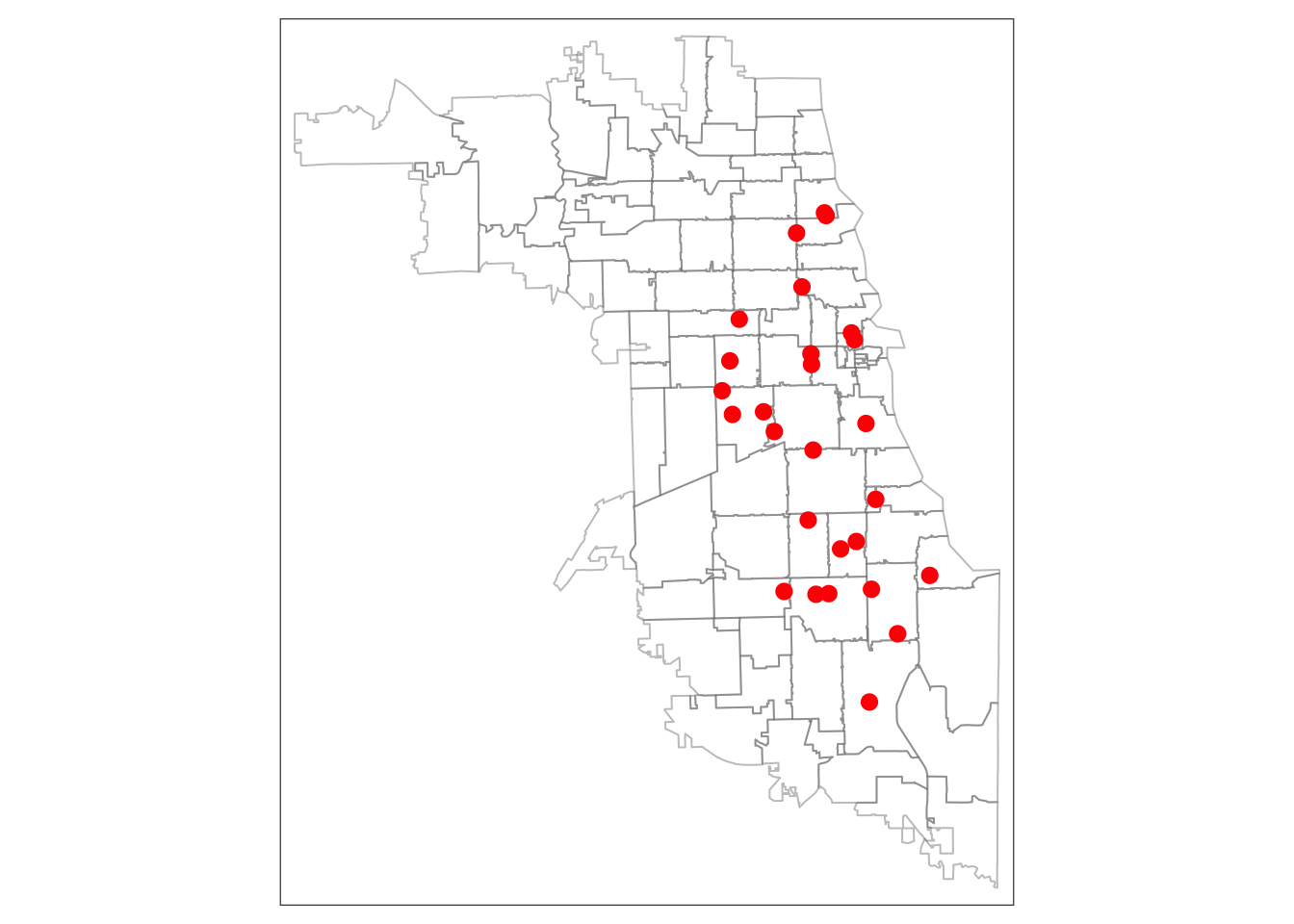
3.4 Spatial Transformation
Next, we check the Coordinate Reference System for our data. Are the coordinate systems for clinic points and community areas the same? For R to treat both coordinate reference systems the same, the metadata has to be exact.
## Coordinate Reference System:
##   User input: WGS 84
##   wkt:
## GEOGCRS["WGS 84",
##     DATUM["World Geodetic System 1984",
##         ELLIPSOID["WGS 84",6378137,298.257223563,
##             LENGTHUNIT["metre",1]]],
##     PRIMEM["Greenwich",0,
##         ANGLEUNIT["degree",0.0174532925199433]],
##     CS[ellipsoidal,2],
##         AXIS["latitude",north,
##             ORDER[1],
##             ANGLEUNIT["degree",0.0174532925199433]],
##         AXIS["longitude",east,
##             ORDER[2],
##             ANGLEUNIT["degree",0.0174532925199433]],
## ID["EPSG",4326]]## Coordinate Reference System:
## User input: WGS 84
## wkt:
## GEOGCRS["WGS 84",
## DATUM["World Geodetic System 1984",
## ELLIPSOID["WGS 84",6378137,298.257223563,
## LENGTHUNIT["metre",1]]],
## PRIMEM["Greenwich",0,
## ANGLEUNIT["degree",0.0174532925199433]],
## CS[ellipsoidal,2],
## AXIS["latitude",north,
## ORDER[1],
## ANGLEUNIT["degree",0.0174532925199433]],
## AXIS["longitude",east,
## ORDER[2],
## ANGLEUNIT["degree",0.0174532925199433]],
## ID["EPSG",4326]]We can see that while both have a code of 4326 and appear to both be WGS84 systems, they are not encoded in exactly the same why. Thus, R will treat them differently – which will pose problems for spatial analysis that interacts these two layers. One way of resolving this challenge is to transform the spatial reference system so that they are exact.
To complicate matters, we are also interested in generating a buffer to approximate a “service area” around each methadone provider. If we want to use a buffer of a mile, we will need to use a spatial data reference system that uses an appropriate distance metric, like feet or meters. As noted in the previous tutorial the WGS84 coordinate reference system uses degrees, and is not an appropriate CRS for the spatial analysis we require.
Thus, our next goal is to transform both spatial data files into a new, standardized CRS.
3.4.1 Transform CRS
To calculate buffers, we will need to convert to a different CRS that preserves distance. Trying using a search engine like Google with search terms “CRS Illinois ft”, for example, to look for a code that provides what we need. After searching, we found EPSG:3435 uses feet for a distance metric. We’ll use that!
First, set a new CRS.
Next, transform both datasets to your new CRS.
Check the CRS of both datasets again. If they are identical you’re ready to move onto the next step!
3.5 Generate Buffers
Now we are ready to generate buffers! We will create a 1-mile buffer to approximate a service area for an urban area. When choosing an appropriate buffer, consider the conceptual model driving your decision. It’s recommended to review literature on common thresholds, consult patients on how they commonly access services, and consider varying travel modes.
We choose a mile as a walkable distance for urban environments, commonly used for acceptable distance to travel for grocery stores in cities. Because methadone providers may be utilized as often as grocery stores for some patients, it may be a reasonable start for analysis.
We use the st_buffer function to create a buffer, and use 5280 feet to equal one mile.
Inspect the structure of the object you just created. Note that this is a new data object, represented as multiple polygons (rather than multiple points). Each buffer around each point is a separate entity.
3.5.1 Visualize buffers
Always visualize a spatial object when calculating one, to confirm it worked correctly. If your buffers are much larger or smaller than expected, it’s often a case of mistaken CRS or projection. Retransform your data, and try again.
We use tmap again, in the static plot mode. We layer our zip code areas, then providers, and then finally the buffers. We use red to color clinics, and blue to color buffers.
## tmap mode set to plottingtm_shape(areas.3435) + tm_borders() +
tm_shape(metClinics.3435) + tm_dots(col = "red") +
tm_shape(metClinic_buffers) + tm_borders(col = "blue") 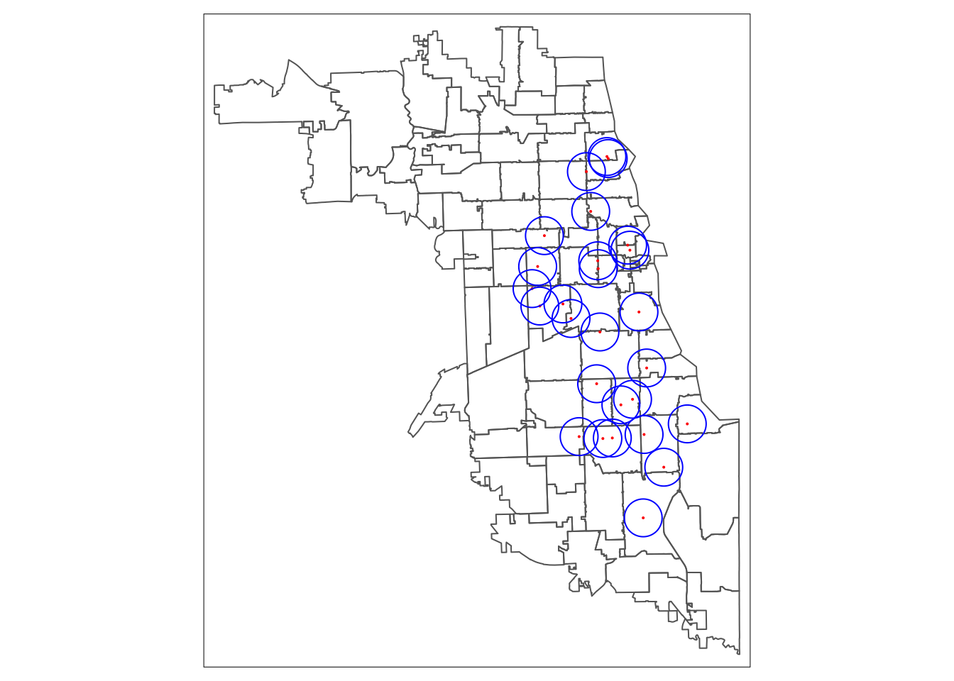
While this map shows our buffers were calculated correctly, the default settings make it difficult to view. To improve aesthetics we change the transparency of zip code boundaries by adjusting the alpha level. We add a fill to the buffers, and make it transparent. We increase the size of the points.
# Map Housing Buffers
tm_shape(areas) + tm_borders(alpha = 0.6) +
  tm_shape(metClinic_buffers) + tm_fill(col = "blue", alpha = .4) + tm_borders(col = "blue") +
tm_shape(metClinics.3435) + tm_dots(col = "red", size = 0.2) 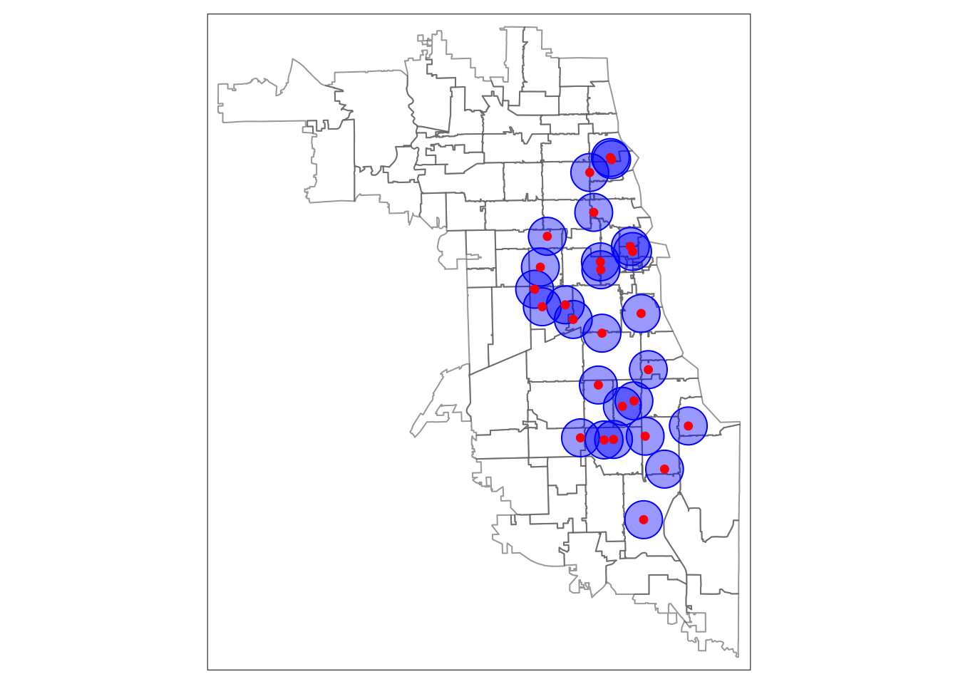
3.5.2 Buffer union
While individual buffers are interesting and can be useful to consider overlapping service areas, we are also interested in getting a sense of which areas fall within a 1-mile service area in our study region – or not. For this, we need to to use a union spatial operation. This will flatten all the individual buffers into one entity.
Inspect the data structures of metClinic_buffers and union.buffers to see what happens to the data in this step.
Finally, we map the buffer union.
tm_shape(areas) +  tm_borders()+
  tm_shape(unionBuffers) + tm_fill(col = "blue", alpha = .2) + tm_borders(col = "blue") +
tm_shape(metClinics.3435) + tm_dots(col = "red", size = 0.4) 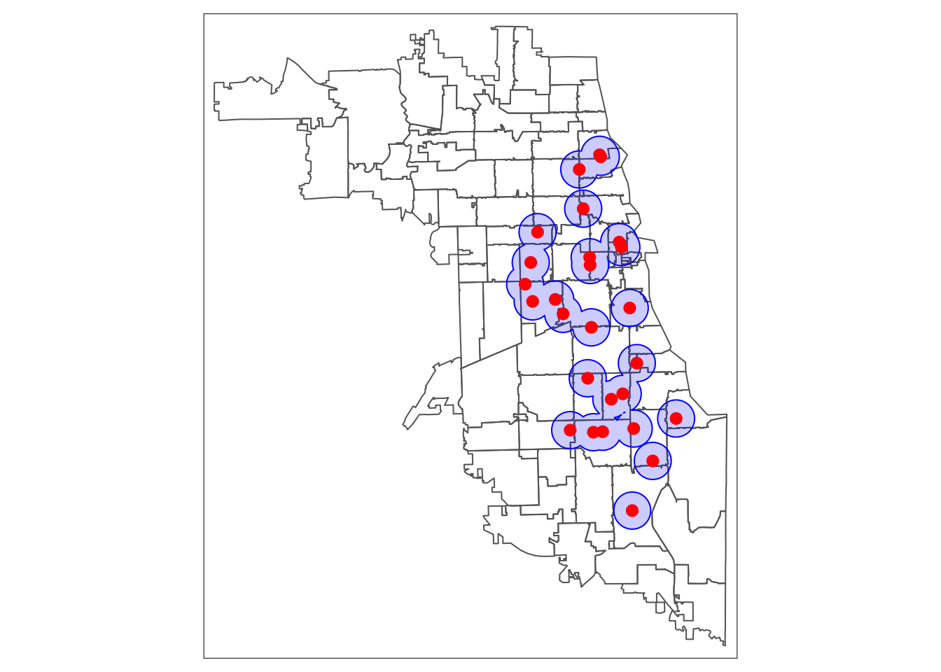
3.6 Rinse & Repeat
From here, we can generate additional buffers to compare access associations and generate multiple visuals.
We generate a two-mile buffer to add:
And then leverage tmap parameter specifications to further customize the a map showing multiple buffers. Here, we add the City of Chicago boundary and soften the zip code boundaries. We add a bounding box for the first zip code layer, so that the whole map is centered around the city boundary (even those the zip codes are layered first). We adjust the transparency of the buffer fills, use different colors, and adjust borders to make the visuals pop. We use the tmap_layout function to take away the frame, add and position a title. Explore the tmap documentation further to find additional options for legends and more. To find color options in R, there are multiple guides online (like this one).
## tmap mode set to plottingtm_shape(areas, bbox=cityBoundary) + tm_borders(alpha = 0.2) +
tm_shape(cityBoundary) + tm_borders(lwd = 1.5) +
tm_shape(metClinic_2mbuffers) + tm_fill(col = "gray10", alpha = .4) + tm_borders(col = "dimgray", alpha = .4) +
tm_shape(metClinic_buffers) + tm_fill(col = "gray90", alpha = .4) + tm_borders(col = "darkslategray") +
tm_shape(metClinics.3435) + tm_dots(col = "red", size = 0.2) +
tm_layout(main.title = "Methadone Clinic Service Areas in Chicago",
main.title.position = "center",
main.title.size = 1,
frame = FALSE)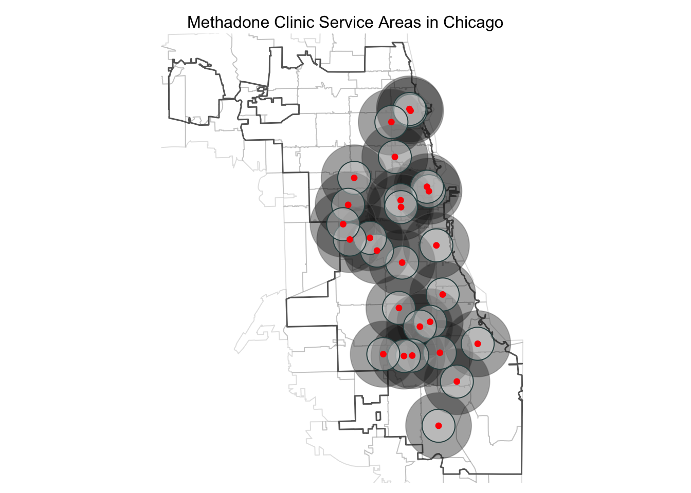
Next, we’ll try an interactive map to better explore the data that we have. We switch the tmap_mode to “view” and focus on our merged 1-mile buffer service areas. We add labels for zip codes using the tm_text parameter, and adjust the size. The resulting map lets us zoom and out to explore the data. Clicking on a point will give additional details about the Methadone provider.
## tmap mode set to interactive viewing