4 Link Community Data
4.1 Overview
Geographic location can serve as a “key” that links different datasets together. By referencing each dataset and enabling its spatial location, we can integrate different types of information in one setting. In this tutorial, we will use the approximated “service areas” generated in our buffer analysis to identify vulnerable populations during the COVID pandemic. We will connect Chicago COVID-19 Case data by ZIP Code, available as a flat file on the city’s data portal, to our environment.
We will then overlap the 1-mile buffers representing walkable access to the Methadone providers in the city. We use a conservative threshold because of the multiple challenges posed by the COVID pandemic that may impact travel.
Our final goal will be to identify zip codes most impacted by COVID that are outside our acceptable access threshold. Our tutorial objectives are to:
- Clean data in preparation of merge
- Integrate data using geographic identifiers
- Generate maps for a basic gap analysis
4.2 Environment Setup
To replicate the codes & functions illustrated in this tutorial, you’ll need to have R and RStudio downloaded and installed on your system. This tutorial assumes some familiarity with the R programming language.
4.2.1 Input/Output
Our inputs include multiple CSV and SHP files, all of which can be found here, though the providers point file was generated in the Geocoding tutorial. Note that all four files are required (.dbf, .prj, .shp, and .shx) to constitute a shapefile.
- Chicago Methadone Clinics,
methadone_clinics.shp - 1-mile buffer zone of Clinics,
methadoneClinics_1mi.shp - Chicago Zip Codes,
chicago_zips.shp - Chicago COVID case data by Zip,
COVID-19_Cases__Tests__and_Deaths_by_ZIP_Code.csv
We will calculate the minimum distance between the resources and the centroids of the zip codes, then save the results as a shapefile and as a CSV. Our final result will be a shapefile/CSV with the minimum distance value for each zip.
4.2.2 Load Libraries
We will use the following packages in this tutorial:
sf: to manipulate spatial datatmap: to visualize and create mapsunits: to convert units within spatial data
Load the libraries for use.
4.2.3 Load data
First we’ll load the shapefiles.
## Reading layer `chicago_zips' from data source `/Users/yashbansal/Desktop/CSDS_RA/opioid-environment-toolkit/data/chicago_zips.shp' using driver `ESRI Shapefile'
## Simple feature collection with 85 features and 9 fields
## geometry type: MULTIPOLYGON
## dimension: XY
## bbox: xmin: -88.06058 ymin: 41.58152 xmax: -87.52366 ymax: 42.06504
## geographic CRS: WGS 84## Reading layer `methadone_clinics' from data source `/Users/yashbansal/Desktop/CSDS_RA/opioid-environment-toolkit/data/methadone_clinics.shp' using driver `ESRI Shapefile'
## Simple feature collection with 27 features and 8 fields
## geometry type: POINT
## dimension: XY
## bbox: xmin: -87.7349 ymin: 41.68698 xmax: -87.57673 ymax: 41.96475
## geographic CRS: WGS 84## Reading layer `methadoneClinics_1mi' from data source `/Users/yashbansal/Desktop/CSDS_RA/opioid-environment-toolkit/data/methadoneClinics_1mi.shp' using driver `ESRI Shapefile'
## Simple feature collection with 1 feature and 1 field
## geometry type: MULTIPOLYGON
## dimension: XY
## bbox: xmin: 1141979 ymin: 1824050 xmax: 1195960 ymax: 1935751
## projected CRS: NAD83 / Illinois East (ftUS)Next, we’ll load some new data we’re interested in joining in: Chicago COVID-19 Cases, Tests, and Deaths by ZIP Code, found on the city data portal here. We’ll load in a CSV and inspect the data:
4.3 Clean & Merge Data
First, let’s inspect COVID case data. What information do we need from this file? We may not need everything, so consider just identifying the field with the geographic identifier and main variable(s) of interest.
## ZIP.Code Week.Number Week.Start Week.End Cases...Weekly
## 1 60603 39 09/20/2020 09/26/2020 0
## 2 60604 39 09/20/2020 09/26/2020 0
## 3 60611 16 04/12/2020 04/18/2020 8
## 4 60611 15 04/05/2020 04/11/2020 7
## 5 60615 11 03/08/2020 03/14/2020 NA
## 6 60603 10 03/01/2020 03/07/2020 NA
## Cases...Cumulative Case.Rate...Weekly Case.Rate...Cumulative
## 1 13 0 1107.3
## 2 31 0 3964.2
## 3 72 25 222.0
## 4 64 22 197.4
## 5 NA NA NA
## 6 NA NA NA
## Tests...Weekly Tests...Cumulative Test.Rate...Weekly
## 1 25 327 2130
## 2 12 339 1534
## 3 101 450 312
## 4 59 349 182
## 5 6 9 14
## 6 0 0 0
## Test.Rate...Cumulative Percent.Tested.Positive...Weekly
## 1 27853.5 0.0
## 2 43350.4 0.0
## 3 1387.8 0.1
## 4 1076.3 0.1
## 5 21.7 NA
## 6 0.0 NA
## Percent.Tested.Positive...Cumulative Deaths...Weekly
## 1 0.0 0
## 2 0.1 0
## 3 0.2 0
## 4 0.2 0
## 5 NA 0
## 6 NA 0
## Deaths...Cumulative Death.Rate...Weekly Death.Rate...Cumulative
## 1 0 0 0
## 2 0 0 0
## 3 0 0 0
## 4 0 0 0
## 5 0 0 0
## 6 0 0 0
## Population Row.ID ZIP.Code.Location
## 1 1174 60603-39 POINT (-87.625473 41.880112)
## 2 782 60604-39 POINT (-87.629029 41.878153)
## 3 32426 60611-16 POINT (-87.620291 41.894734)
## 4 32426 60611-15 POINT (-87.620291 41.894734)
## 5 41563 60615-11 POINT (-87.602725 41.801993)
## 6 1174 60603-10 POINT (-87.625473 41.880112)From this we can assess the need for the following variables: ZIP Code and Percent Tested Positive - Cumulative. Let’s subset the data accordingly. Because this data file has extremely long header names (common in the epi world), let’s use the colnames function to get exactly what we need.
## [1] "ZIP.Code"
## [2] "Week.Number"
## [3] "Week.Start"
## [4] "Week.End"
## [5] "Cases...Weekly"
## [6] "Cases...Cumulative"
## [7] "Case.Rate...Weekly"
## [8] "Case.Rate...Cumulative"
## [9] "Tests...Weekly"
## [10] "Tests...Cumulative"
## [11] "Test.Rate...Weekly"
## [12] "Test.Rate...Cumulative"
## [13] "Percent.Tested.Positive...Weekly"
## [14] "Percent.Tested.Positive...Cumulative"
## [15] "Deaths...Weekly"
## [16] "Deaths...Cumulative"
## [17] "Death.Rate...Weekly"
## [18] "Death.Rate...Cumulative"
## [19] "Population"
## [20] "Row.ID"
## [21] "ZIP.Code.Location"4.3.1 Subset Data
We can now subset to just include the fields we need. There are many different ways to subset in R – we just use one example here! Inspect your data to confirm it was pulled correctly.
## ZIP.Code Case.Rate...Cumulative
## 1 60603 1107.3
## 2 60604 3964.2
## 3 60611 222.0
## 4 60611 197.4
## 5 60615 NA
## 6 60603 NA4.3.2 Identify Geographic Key
Before merging, we need to first identify the geographic identifier we would like to merge on. It is the field “ZIP.Code” in our subset. What about the zip code file, which we will be merging to?
## Simple feature collection with 6 features and 9 fields
## geometry type: MULTIPOLYGON
## dimension: XY
## bbox: xmin: -88.06058 ymin: 41.73452 xmax: -87.58209 ymax: 42.04052
## geographic CRS: WGS 84
## ZCTA5CE10 GEOID10 CLASSFP10 MTFCC10 FUNCSTAT10 ALAND10
## 1 60501 60501 B5 G6350 S 12532295
## 2 60007 60007 B5 G6350 S 36493383
## 3 60651 60651 B5 G6350 S 9052862
## 4 60652 60652 B5 G6350 S 12987857
## 5 60653 60653 B5 G6350 S 6041418
## 6 60654 60654 B5 G6350 S 1464813
## AWATER10 INTPTLAT10 INTPTLON10
## 1 974360 +41.7802209 -087.8232440
## 2 917560 +42.0086000 -087.9973398
## 3 0 +41.9020934 -087.7408565
## 4 0 +41.7479319 -087.7147951
## 5 1696670 +41.8199645 -087.6059654
## 6 113471 +41.8918225 -087.6383036
## geometry
## 1 MULTIPOLYGON (((-87.86289 4...
## 2 MULTIPOLYGON (((-88.06058 4...
## 3 MULTIPOLYGON (((-87.77559 4...
## 4 MULTIPOLYGON (((-87.74205 4...
## 5 MULTIPOLYGON (((-87.62623 4...
## 6 MULTIPOLYGON (((-87.64775 4...Aha – in this dataset, the zip is identified as either the ZCTA5CE10 field or GEOID10 field. Not that we are actually working with 5-digit ZCTA fields, not 9-digit ZIP codes… We decide to merge on the GEOID10 field. To make our lives easier, we’ll generate a duplicate field in our subset with a new name, GEOID10, to match. We also convert from the factor structure to a character field to match the data structure of the master zip file.
4.3.3 Merge Data
Let’s merge the data using the zip code geographic identifier, “ZIP Code” field, to bring in the the Percent Tested Positive - Cumalative dataset. Inspect the data to confirm it merged correctly!
## Simple feature collection with 6 features and 11 fields
## geometry type: MULTIPOLYGON
## dimension: XY
## bbox: xmin: -87.63396 ymin: 41.88083 xmax: -87.6129 ymax: 41.88893
## geographic CRS: WGS 84
## GEOID10 ZCTA5CE10 CLASSFP10 MTFCC10 FUNCSTAT10 ALAND10 AWATER10
## 1 60601 60601 B5 G6350 S 934226 60682
## 2 60601 60601 B5 G6350 S 934226 60682
## 3 60601 60601 B5 G6350 S 934226 60682
## 4 60601 60601 B5 G6350 S 934226 60682
## 5 60601 60601 B5 G6350 S 934226 60682
## 6 60601 60601 B5 G6350 S 934226 60682
## INTPTLAT10 INTPTLON10 ZIP.Code Case.Rate...Cumulative
## 1 +41.8856419 -087.6215226 60601 1451.4
## 2 +41.8856419 -087.6215226 60601 872.2
## 3 +41.8856419 -087.6215226 60601 919.9
## 4 +41.8856419 -087.6215226 60601 558.8
## 5 +41.8856419 -087.6215226 60601 156.7
## 6 +41.8856419 -087.6215226 60601 477.0
## geometry
## 1 MULTIPOLYGON (((-87.63396 4...
## 2 MULTIPOLYGON (((-87.63396 4...
## 3 MULTIPOLYGON (((-87.63396 4...
## 4 MULTIPOLYGON (((-87.63396 4...
## 5 MULTIPOLYGON (((-87.63396 4...
## 6 MULTIPOLYGON (((-87.63396 4...4.4 Visualize Data
Now we are ready to visualize our data! First we’ll make a simple map. We generate a choropleth map of case rate data using quantile bins, and the Blue-Purple color palette. You can find an R color cheatsheet useful for identifying palette codes here. (More details on thematic mapping are in tutorials that follow!) We overlay the buffers and clincal providers.
## tmap mode set to plottingtm_shape(zipsMerged) +
tm_polygons("Case.Rate...Cumulative", style="quantile", pal="BuPu",
title = "COVID Case Rate") +
tm_shape(buffers) + tm_borders(col = "blue") +
tm_shape(methadoneSf) + tm_dots(col = "black", size = 0.2) 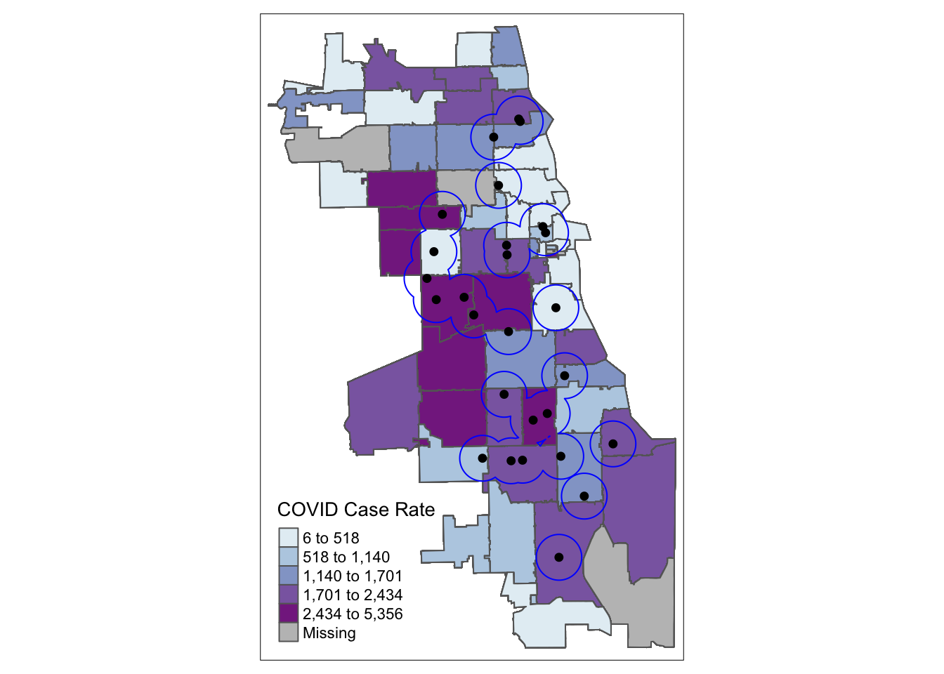
Already we can generate some insight. Areas on the far West side of the city have some of the highest case rates, but are outside a walkable distance to Methadone providers. For individuals with opioid use disorder requiring medication access in these locales, they may be especially vulnerable during the pandemic.
Next, we adjust some tmap parameters to improve our map. Now we switch to a red-yellow-green palette, and specify six bins for our quantile map. We flip the direction of the palette using a negative sign, so that red corresponds to areas with higher rates. We adjust transparency using an alpha parameter, and line thickness using the lwd parameter.
tm_shape(zipsMerged) +
tm_fill("Case.Rate...Cumulative", style="quantile", n=6, pal="-RdYlGn",
title = "COVID Case Rate",alpha = 0.8) +
tm_borders(lwd = 0) +
tm_shape(buffers) + tm_borders(col = "gray") + tm_fill(alpha=0.5) +
tm_shape(methadoneSf) + tm_dots(col = "black", size = 0.1) +
tm_layout(main.title = "Walkable Methadone Service Areas",
main.title.position = "center",
main.title.size = 1,
frame = FALSE)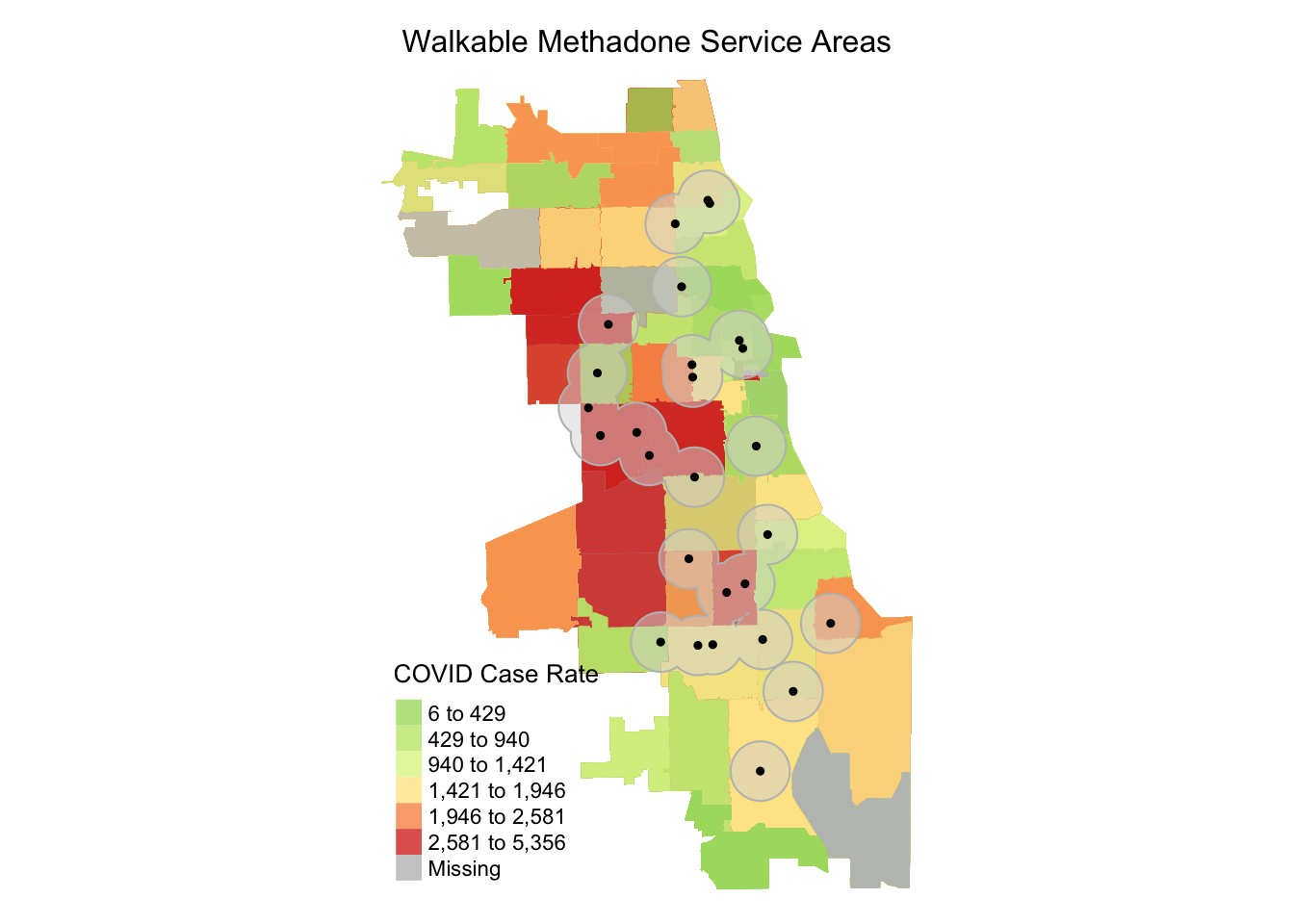
To improve our map even further, let’s make it interactive! By switching the tmap_mode function to “view” (from “plot” the default), our newly rendered map is not interactive. We can zoom in and out, click on different basemaps or turn layers on our off, and click on resources for more information.
## tmap mode set to interactive viewing