5 Census Data Wrangling
5.1 Overview
Once we identify the appropriate access metric to use, we can now include contextual data to add nuance to our findings. This can help identify if any specific disparities in access exist for certain groups of people or if there are any specific factors that can help explain the spatial patterns. Such datasets are often sourced from the US Census Bureau. The American Community Survey (ACS) is an ongoing survey that provides data every year with 1 and 5-year estimates. We generally recommend using the 5-year estimates as these multiperiod estimates tend to have increased statistical reliability as compared to the 1-year numbers, especially for less populated areas and small population subgroups.
In this tutorial we demonstrate how to explore and download most commonly used population datasets from the same, with and without spatial components. Please note this tutorial focuses only on the American Community Survey datasets available via the Census Bureau API. More details about using tidycensus, with tutorials generated by package authors, can be found here.
Our objectives are to:
- Download census data through the Census API
- Download census boundaries thorough the Census API
- Wrangle, clean and merge data for further integration
5.2 Environment Setup
To replicate the codes & functions illustrated in this tutorial, you’ll need to have R and RStudio downloaded and installed on your system. This tutorial assumes some familiarity with the R programming language.
5.2.1 Input/Output
Our only external input will be the SHP file for Chicago City Boundary to filter the zipcode level data for the City of Chicago, which can be found here. Simply downloading the datasets from the US Census Bureau website doesn’t require any external file input.
- Chicago City Boundary,
boundaries_chicago.geojson
Our output will be two sets of files:
- CSV file and shapefile with Race Data distributions at county level for the state of Illinois.
- and CSV file and shapefile with Population and Per Capita Income for the zipcodes within the city of Chicago for 2018.
5.2.2 Load Libraries
We will use the following packages in this tutorial:
sf: to read/write sf (spatial) objectstidycensus: to download census variables using ACS APItidyverse: to manipulate and clean datatigris: to download census tiger shapefiles
Load the required libraries.
5.3 Enable Census API Key
To be able to use the Census API, we need to signup for an API key. This key effectively is a string identifier for the server to communicate with your machine. A key can be obtained using an email from here. Once we get the key, we can install it by running the code below.
In instances where we might not want to save our key in the .Renviron - for example, when using a shared computer, we can always reinstall the same key using the code above but with install = FALSE.
To check an already installed census API key, run
5.4 Load Data Dynamically
We can now start using the tidycensus package to download population based datasets from the US Census Bureau. In this tutorial, we will be covering methods to download data at the state, county, zip and census tract levels. We will also be covering methods to download the data with and without the geometry feature of the geographic entities.
To download a particular variable or table using tidycensus, we need the relevant variable ID, which one can check by reviewing the variables available via load_variables() function. For details on exploring the variables available via the tidycensus & to get their identifiers, check the Explore variables available section in Appendix.
We can now download the variables using get_acs() function. Given ACS data is based of an annual sample, the datapoints are available as an estimate with a margin or error (moe). The package provides both values for any requested variable in the tidy format.
For the examples covered in this tutorial, the 4 main inputs for get_acs() function are:
geography- for what scale to source the data for (state / county / tract / zcta)variables- character string or a vector of character strings of variable IDs to sourceyear- the year to source the data forgeometry- whether or not to include the geometry feature in the tibble. (TRUE / FALSE)
5.4.1 State Level
To get data for only a specific state, we can add state = sampleStateName.
stateDf <- get_acs(geography = 'state', variables = c(totPop18 = "B01001_001",
                                                      hispanic ="B03003_003",
                                                      notHispanic = "B03003_002",
                                                      white = "B02001_002",
                                                      afrAm = "B02001_003",
                                                      asian = "B02001_005"),
                   year = 2018, geometry = FALSE)
head(stateDf)
## # A tibble: 6 x 5
## GEOID NAME variable estimate moe
## <chr> <chr> <chr> <dbl> <dbl>
## 1 01 Alabama totPop18 4864680 NA
## 2 01 Alabama white 3317453 3345
## 3 01 Alabama afrAm 1293186 2745
## 4 01 Alabama asian 64609 1251
## 5 01 Alabama notHispanic 4661534 393
## 6 01 Alabama hispanic 203146 393As we can see the data is available in the tidy format. We can use other tools in the tidyverse universe to clean and manipulate it.
stateDf <- stateDf %>%
            select(GEOID, NAME, variable, estimate) %>%
            spread(variable, estimate) %>%
            mutate(hispPr18  = hispanic/totPop18, whitePr18 = white/totPop18,
                   afrAmPr18 = afrAm/totPop18, asianPr18 = asian/totPop18) %>%
            select(GEOID,totPop18,hispPr18,whitePr18,afrAmPr18, asianPr18)

head(stateDf)
## # A tibble: 6 x 6
## GEOID totPop18 hispPr18 whitePr18 afrAmPr18 asianPr18
## <chr> <dbl> <dbl> <dbl> <dbl> <dbl>
## 1 01 4864680 0.0418 0.682 0.266 0.0133
## 2 02 738516 0.0693 0.648 0.0327 0.0630
## 3 04 6946685 0.311 0.772 0.0439 0.0329
## 4 05 2990671 0.0732 0.770 0.154 0.0147
## 5 06 39148760 0.389 0.601 0.0579 0.143
## 6 08 5531141 0.214 0.842 0.0412 0.03125.4.2 County Level
Similarly, for county level
- use
geometry = countyto download for all counties in the U.S. - use
geometry = county, state = sampleStateNamefor all counties within a state - use
geometry = county, state = sampleStateName, county = sampleCountyNamefor a specific county
countyDf <- get_acs(geography = 'county', variables = c(totPop18 = "B01001_001",
                                                        hispanic ="B03003_003",
                                                        notHispanic = "B03003_002",
                                                        white = "B02001_002",
                                                        afrAm = "B02001_003",
                                                        asian = "B02001_005"),
                    year = 2018, state = 'IL', geometry = FALSE) %>%
            select(GEOID, NAME, variable, estimate) %>%
            spread(variable, estimate) %>%
            mutate(hispPr18  = hispanic/totPop18, whitePr18 = white/totPop18,
                   afrAmPr18 = afrAm/totPop18, asianPr18 = asian/totPop18) %>%
            select(GEOID,totPop18,hispPr18,whitePr18,afrAmPr18, asianPr18)

head(countyDf)
## # A tibble: 6 x 6
## GEOID totPop18 hispPr18 whitePr18 afrAmPr18 asianPr18
## <chr> <dbl> <dbl> <dbl> <dbl> <dbl>
## 1 17001 66427 0.0154 0.931 0.0408 0.00813
## 2 17003 6532 0.0112 0.624 0.332 0.000919
## 3 17005 16712 0.0346 0.909 0.0624 0.0117
## 4 17007 53606 0.214 0.874 0.0222 0.0118
## 5 17009 6675 0.0428 0.774 0.204 0.00554
## 6 17011 33381 0.0897 0.936 0.00932 0.008665.4.3 Census Tract Level
For census tract level, at the minimum stateName needs to be provided.
- use
geometry = tract, state = sampleStateNameto download all tracts within a state - use
geometry = tract, state = sampleStateName, county = sampleCountyNameto download all tracts within a specific county
tractDf <- get_acs(geography = 'tract',variables = c(totPop18 = "B01001_001",
                                                   hispanic ="B03003_003",
                                                   notHispanic = "B03003_002",
                                                   white = "B02001_002",
                                                   afrAm = "B02001_003",
                                                   asian = "B02001_005"),
                    year = 2018, state = 'IL', geometry = FALSE) %>%
            select(GEOID, NAME, variable, estimate) %>%
            spread(variable, estimate) %>%
            mutate(hispPr18  = hispanic/totPop18, whitePr18 = white/totPop18,
                   afrAmPr18 = afrAm/totPop18, asianPr18 = asian/totPop18) %>%
            select(GEOID,totPop18,hispPr18,whitePr18,afrAmPr18, asianPr18)

head(tractDf)
5.4.4 Zipcode Level
For zipcode level, use geometry = zcta. Given zips cross county/state lines, zcta data is only available for the entire U.S.
zctaDf <- get_acs(geography = 'zcta',variables = c(totPop18 = "B01001_001",
                                                   hispanic ="B03003_003",
                                                   notHispanic = "B03003_002",
                                                   white = "B02001_002",
                                                   afrAm = "B02001_003",
                                                   asian = "B02001_005"),
                    year = 2018, geometry = FALSE) %>%
            select(GEOID, NAME, variable, estimate) %>%
            spread(variable, estimate) %>%
            mutate(hispPr18  = hispanic/totPop18, whitePr18 = white/totPop18,
                   afrAmPr18 = afrAm/totPop18, asianPr18 = asian/totPop18) %>%
            select(GEOID,totPop18,hispPr18,whitePr18,afrAmPr18, asianPr18)
Inspect the data.
## # A tibble: 6 x 6
##   GEOID totPop18 hispPr18 whitePr18 afrAmPr18 asianPr18
##   <chr>    <dbl>    <dbl>     <dbl>     <dbl>     <dbl>
## 1 00601    17242    0.997     0.755   0.00841  0.000174
## 2 00602    38442    0.935     0.794   0.0278   0
## 3 00603    48814    0.974     0.765   0.0395   0.00746
## 4 00606     6437    0.998     0.408   0.0231   0
## 5 00610    27073    0.962     0.755   0.0257   0
## 6 00612 60303 0.993 0.807 0.0456 0.00985## [1] 33120 6Given zipcode data can only be sourced for the entire nation, after sourcing it, we can filter them for certain region,e.g. below we can filter for zipcodes in Chicago by using str_detect. If we had the geometry information, we could overlay the zipcode geometry with the desired shape boundary to easily filter the required region. We will illustrate that in the Get Geometry section.
zipChicagoDf <- get_acs(geography = 'zcta', variables = c(perCapInc = "DP03_0088"),year = 2018, geometry = FALSE) %>%
                  select(GEOID, NAME, variable, estimate) %>%
                  filter(str_detect( GEOID,"^606")) %>%  ## add a str filter
                  spread(variable, estimate) %>%
                  select(GEOID, perCapInc)
## Getting data from the 2014-2018 5-year ACS## Using the ACS Data Profile5.4.5 Save Data
And now we can save the county and zipcode datasets in CSV file using the code below.
write.csv(countyDf, "data/ilcounty_18_race.csv")
write.csv(zipChicagoDf , file = "data/chizips_18_pci.csv")
For more details on the other geographies available via the tidycensus package, check here.
5.5 Get Geometry
Geometry/Geographic Boundaries are one of the key features for American Community Survey Data as they set up the framework for data collection and estimation. While boundaries don’t change often, updates do occur from time to time and census data for a specific year generally tends to use the boundaries available at the beginning of that year. Most ACS products since 2010 reflect the 2010 Census Geographic Definitions. Given certain boundaries like congressional districts, census tracts & block groups are updated after every decennial census, products for year 2009 and earlier will have significantly different boundaries from that in 2010. We recommend using IPUMS datasets to generate estimates for years prior to 2010.
The datasets downloaded so far did not have a spatial geometry feature attached to them. To run any spatial analysis on the race data above, we would need to join these dataframes to another spatially-enabled sf object. We can do so by joining on the ‘GEOID’ or any other identifier. We can download the geometry information using two methods :
- using
tigris - using
tidycensus
5.5.1 Using tigris
To download and use the Tiger Shapefiles shared by the US Census Bureau we will use the tigris package. Set cb = TRUE to get generalized files, these don’t have high resolution details and hence are smaller in size.
yearToFetch <- 2018

stateShp <- states(year = yearToFetch, cb = TRUE)
countyShp <- counties(year = yearToFetch, state = 'IL', cb = TRUE)
tractShp <- tracts(state = 'IL',year = yearToFetch, cb = TRUE)
zctaShp <- zctas(year = yearToFetch, cb = TRUE)
Sometimes the ACS FTP might be down for system maintenance or some other reason, and in such a scenario the code returns an error message like below. You can check the website status from here to confirm. If the website is truly down, we recommend trying the download again in a few hours.
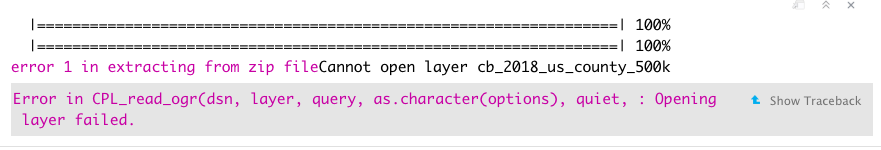
Figure 5.1: R error message

Figure 5.2: ACS website outage message
After we have successfully download the geometry files, we can now merge these shapes with the race data downloaded in previous section.
For states:
# check object types & identifier variable type
# str(stateShp)
# str(stateDf)
stateShp <- merge(stateShp, stateDf, by.x  = 'STATEFP', by.y = 'GEOID', all.x = TRUE)
head(stateShp)
## Simple feature collection with 6 features and 14 fields
## geometry type: MULTIPOLYGON
## dimension: XY
## bbox: xmin: -179.1489 ymin: 30.22333 xmax: 179.7785 ymax: 71.36516
## geographic CRS: NAD83
## STATEFP STATENS AFFGEOID GEOID STUSPS NAME LSAD
## 1 01 01779775 0400000US01 01 AL Alabama 00
## 2 02 01785533 0400000US02 02 AK Alaska 00
## 3 04 01779777 0400000US04 04 AZ Arizona 00
## 4 05 00068085 0400000US05 05 AR Arkansas 00
## 5 06 01779778 0400000US06 06 CA California 00
## 6 08 01779779 0400000US08 08 CO Colorado 00
## ALAND AWATER totPop18 hispPr18 whitePr18
## 1 1.311740e+11 4593327154 4864680 0.04175938 0.6819468
## 2 1.478840e+12 245481577452 738516 0.06930926 0.6483732
## 3 2.941986e+11 1027337603 6946685 0.31141645 0.7721872
## 4 1.347689e+11 2962859592 2990671 0.07324510 0.7700192
## 5 4.035039e+11 20463871877 39148760 0.38881377 0.6010169
## 6 2.684229e+11 1181621593 5531141 0.21420427 0.8417041
## afrAmPr18 asianPr18 geometry
## 1 0.26583167 0.01328124 MULTIPOLYGON (((-88.05338 3...
## 2 0.03267228 0.06303993 MULTIPOLYGON (((179.4825 51...
## 3 0.04394312 0.03294910 MULTIPOLYGON (((-114.8163 3...
## 4 0.15413598 0.01470840 MULTIPOLYGON (((-94.61783 3...
## 5 0.05792968 0.14315496 MULTIPOLYGON (((-118.6044 3...
## 6 0.04120994 0.03122231 MULTIPOLYGON (((-109.0603 3...Similarly for counties, zctas & census tracts we can use the code below.
countyShp <- merge(countyShp, countyDf, by.x  = 'GEOID', by.y = 'GEOID', all.x = TRUE) %>%
                select(GEOID,totPop18,hispPr18,whitePr18,afrAmPr18, asianPr18)

tractShp <- merge(tractShp, tractDf, by.x  = 'GEOID', by.y = 'GEOID', all.x = TRUE) %>%
              select(GEOID,totPop18,hispPr18,whitePr18,afrAmPr18, asianPr18)

zctaShp <- merge(zctaShp, zctaDf, by.x  = 'GEOID10', by.y = 'GEOID', all.x = TRUE)%>%
              select(GEOID10,totPop18,hispPr18,whitePr18,afrAmPr18, asianPr18)
5.5.2 Using tidycensus
The previous method adds an additional step of using tigris package to download the shapefile.
The tidycensus package already has the wrapper for invoking tigris within the get_acs() function, and we can simply download the dataset with geometry feature by using geometry = TRUE.
The wrapper adds the geometry information to each variable sourced, and the file size can become large in the intermediary steps and slow down the performance, even though the data is in tidy format. So if you are looking to download many variables with large API requests, we recommend downloading the dataset without geometry information and then downloading a nominal variable like total population or per capita income with get geometry using get_acs() or simply using the tigris method, as covered in previous section & then implementing a merge. We have illustrated both methods below.
tractDf <- get_acs(geography = 'tract', variables = c(totPop18 = "B01001_001",
                                                      hispanic ="B03003_003",
                                                      notHispanic = "B03003_002",
                                                      white = "B02001_002",
                                                      afrAm = "B02001_003",
                                                      asian = "B02001_005"),
                   year = 2018, state  = 'IL', geometry = FALSE) %>%
            select(GEOID, NAME, variable, estimate) %>%
            spread(variable, estimate) %>%
            mutate(hispPr18  = hispanic/totPop18, whitePr18 = white/totPop18,
                   afrAmPr18 = afrAm/totPop18, asianPr18 = asian/totPop18) %>%
            select(GEOID,totPop18,hispPr18,whitePr18,afrAmPr18, asianPr18)

tractShp <- get_acs(geography = 'tract', variables = c(perCapitaIncome = "DP03_0088"),
                    year = 2018, state  = 'IL', geometry = TRUE) %>%
            select(GEOID, NAME, variable, estimate) %>%
            spread(variable, estimate)


tractsShp <- merge(tractShp, tractDf, by.x = 'GEOID', by.y = 'GEOID', all.x = TRUE)
head(tractShp)
## Simple feature collection with 6 features and 3 fields
## geometry type: MULTIPOLYGON
## dimension: XY
## bbox: xmin: -88.79336 ymin: 41.7943 xmax: -87.63536 ymax: 41.95088
## geographic CRS: NAD83
## GEOID NAME
## 1 17031843800 Census Tract 8438, Cook County, Illinois
## 2 17037001002 Census Tract 10.02, DeKalb County, Illinois
## 3 17031243000 Census Tract 2430, Cook County, Illinois
## 4 17031250600 Census Tract 2506, Cook County, Illinois
## 5 17031251700 Census Tract 2517, Cook County, Illinois
## 6 17031260400 Census Tract 2604, Cook County, Illinois
## perCapitaIncome geometry
## 1 19331 MULTIPOLYGON (((-87.64554 4...
## 2 11308 MULTIPOLYGON (((-88.79317 4...
## 3 48843 MULTIPOLYGON (((-87.68195 4...
## 4 22905 MULTIPOLYGON (((-87.7756 41...
## 5 14739 MULTIPOLYGON (((-87.74826 4...
## 6 12610 MULTIPOLYGON (((-87.74061 4...To get zipcode level data for a specific region, we first need to download the required dataset for the entire country and then we can filter the relevant zipcodes by overlaying the downloaded dataset with the geometry feature of that region. For example, to get data only for Chicago, we can overlay the city boundaries over the zcta file(with geometry) using the st_intersection function as shown below.
zctaShp <- get_acs(geography = 'zcta', variables = c(totPop18 = "B01001_001",
                                                           perCapInc = "DP03_0088"),
                         year = 2018, geometry = TRUE) %>%
                  select(GEOID, NAME, variable, estimate) %>%
                  spread(variable, estimate) %>%
                  rename(totPop18 = B01001_001, perCapitaInc = DP03_0088) %>%
                  select(GEOID,totPop18,perCapitaInc)
head(zctaShp)
## Simple feature collection with 6 features and 3 fields
## geometry type: MULTIPOLYGON
## dimension: XY
## bbox: xmin: -67.23935 ymin: 18.11083 xmax: -66.57805 ymax: 18.51298
## geographic CRS: NAD83
## # A tibble: 6 x 4
## GEOID totPop18 perCapitaInc geometry
## <chr> <dbl> <dbl> <MULTIPOLYGON [°]>
## 1 00601 17242 6999 (((-66.83526 18.20998, -66.83287 18…
## 2 00602 38442 9277 (((-67.23935 18.37626, -67.2381 18.…
## 3 00603 48814 11307 (((-67.16965 18.47511, -67.16909 18…
## 4 00606 6437 5943 (((-67.05123 18.17743, -67.04986 18…
## 5 00610 27073 10220 (((-67.22403 18.29949, -67.22265 18…
## 6 00612 60303 10549 (((-66.68181 18.44724, -66.6819 18.…## Reading layer `boundaries_chicago' from data source `/Users/yashbansal/Desktop/CSDS_RA/opioid-environment-toolkit/data/boundaries_chicago.geojson' using driver `GeoJSON'
## Simple feature collection with 1 feature and 4 fields
## geometry type: MULTIPOLYGON
## dimension: XY
## bbox: xmin: -87.94011 ymin: 41.64454 xmax: -87.52414 ymax: 42.02304
## geographic CRS: WGS 84# set same CRS for both shapefiles
chiCityBoundary <- st_transform(chiCityBoundary, 4326)
zctaShp <- st_transform(zctaShp, 4326)
#only keep those zipcodes that intersect the Chicago city boundary
zipChicagoShp <- st_intersection(zctaShp,chiCityBoundary)## Warning: attribute variables are assumed to be spatially constant
## throughout all geometries## Simple feature collection with 6 features and 7 fields
## geometry type: GEOMETRY
## dimension: XY
## bbox: xmin: -87.94011 ymin: 41.68284 xmax: -87.52454 ymax: 42.01914
## geographic CRS: WGS 84
## # A tibble: 6 x 8
## GEOID totPop18 perCapitaInc name objectid shape_area shape_len
## <chr> <dbl> <dbl> <chr> <chr> <chr> <chr>
## 1 46320 13703 17983 CHIC… 1 645027662… 845282.9…
## 2 60007 33420 39312 CHIC… 1 645027662… 845282.9…
## 3 60018 30386 25607 CHIC… 1 645027662… 845282.9…
## 4 60068 37736 53792 CHIC… 1 645027662… 845282.9…
## 5 60076 31867 37700 CHIC… 1 645027662… 845282.9…
## 6 60077 28329 30903 CHIC… 1 645027662… 845282.9…
## # … with 1 more variable: geometry <GEOMETRY [°]>5.5.3 Save Data
We previously saved our files without geometry information as CSVs. Now we can save the census tract race data and Chicago zipcode level per capita income with geometries as shapefiles using write_sf.
## Warning in abbreviate_shapefile_names(obj): Field names
## abbreviated for ESRI Shapefile driver
5.6 Appendix
5.6.1 Explore variables
Using tidycensus we can download datasets from various types of tables. The ones most commonly used are:
- Data Profiles - These are the most commonly used collection of variables grouped by category, e.g. Social (DP02), Economic (DP03), Housing (DP04), Demographic (DP05)
- Subject Profiles - These generally have more detailed information variables (than DP) grouped by category, e.g. Age & Sex (S0101), Disability Characteristics (S1810)
- The package also allows access to a suite of B & C tables.
We can explore all the variables for our year of interest by running the code below. Please note as the Profiles evolve, variable IDs might change from year to year.
sVarNames <- load_variables(2018, "acs5/subject", cache = TRUE)
pVarNames <- load_variables(2018, "acs5/profile", cache = TRUE)
otherVarNames <- load_variables(2018, "acs5", cache = TRUE)

head(pVarNames)
## # A tibble: 6 x 3
## name label concept
## <chr> <chr> <chr>
## 1 DP02_00… Estimate!!HOUSEHOLDS BY TYPE… SELECTED SOCIAL CHARACTE…
## 2 DP02_00… Percent Estimate!!HOUSEHOLDS… SELECTED SOCIAL CHARACTE…
## 3 DP02_00… Estimate!!HOUSEHOLDS BY TYPE… SELECTED SOCIAL CHARACTE…
## 4 DP02_00… Percent Estimate!!HOUSEHOLDS… SELECTED SOCIAL CHARACTE…
## 5 DP02_00… Estimate!!HOUSEHOLDS BY TYPE… SELECTED SOCIAL CHARACTE…
## 6 DP02_00… Percent Estimate!!HOUSEHOLDS… SELECTED SOCIAL CHARACTE…A tibble with table & variable information has three columns : name, label, concept.
Name is a combination of table id and variable id within that table. Concept generally identifies the table name or grouping used to arrange variables. Label provides textual details about the variable.
We can explore these tibbles to identify the correct variable ID name to use with the get_acs() function by using View(sVarNames) or other filters e.g. for age
sVarNames %>% filter(str_detect(concept, "AGE AND SEX")) %>%  # search for this concept
              filter(str_detect(label, "Under 5 years")) %>%  # search for variables
              mutate(label = sub('^Estimate!!', '', label)) %>% # remove unnecessary text
              select(variableId = name, label) # drop unnecessary columns and rename
## # A tibble: 6 x 2
## variableId label
## <chr> <chr>
## 1 S0101_C01_002 Total!!Total population!!AGE!!Under 5 years
## 2 S0101_C02_002 Percent!!Total population!!AGE!!Under 5 years
## 3 S0101_C03_002 Male!!Total population!!AGE!!Under 5 years
## 4 S0101_C04_002 Percent Male!!Total population!!AGE!!Under 5 years
## 5 S0101_C05_002 Female!!Total population!!AGE!!Under 5 years
## 6 S0101_C06_002 Percent Female!!Total population!!AGE!!Under 5 ye…sVarNames %>% filter(str_sub(name, 1, 5) == "S0101") %>% # search for these tables
filter(str_detect(label, "Under 5 years")) %>% # search for variables
mutate(label = sub('^Estimate!!', '', label)) %>% # remove unnecessary text
select(variableId = name, label) # drop unnecessary columns and rename## # A tibble: 6 x 2
## variableId label
## <chr> <chr>
## 1 S0101_C01_002 Total!!Total population!!AGE!!Under 5 years
## 2 S0101_C02_002 Percent!!Total population!!AGE!!Under 5 years
## 3 S0101_C03_002 Male!!Total population!!AGE!!Under 5 years
## 4 S0101_C04_002 Percent Male!!Total population!!AGE!!Under 5 years
## 5 S0101_C05_002 Female!!Total population!!AGE!!Under 5 years
## 6 S0101_C06_002 Percent Female!!Total population!!AGE!!Under 5 ye…e.g per capita income, we can check on DP table variables.
pVarNames %>% filter(str_detect(label, "Per capita")) %>%  # search for variables
              mutate(label = sub('^Estimate!!', '', label)) %>% # remove unnecessary text
              select(variable = name, label) # drop unnecessary columns and rename
## # A tibble: 2 x 2
## variable label
## <chr> <chr>
## 1 DP03_0088 INCOME AND BENEFITS (IN 2018 INFLATION-ADJUSTED DOLL…
## 2 DP03_0088P Percent Estimate!!INCOME AND BENEFITS (IN 2018 INFLA…pVarNames %>% filter(str_detect(label, "Under 5 years")) %>% # search for variables
mutate(label = sub('^Estimate!!', '', label)) %>% # remove unnecessary text
select(variable = name, label) # drop unnecessary columns and rename## # A tibble: 2 x 2
## variable label
## <chr> <chr>
## 1 DP05_0005 SEX AND AGE!!Total population!!Under 5 years
## 2 DP05_0005P Percent Estimate!!SEX AND AGE!!Total population!!Und…The order and structure of profile tables can change from year to year, hence the variable Id or label, so when downloading same dataset over different years we recommend using the standard B & C tables.
otherVarNames %>% filter(str_detect(label, "Per capita")) %>%  # search for variables
              mutate(label = sub('^Estimate!!', '', label)) %>% # remove unnecessary text
              select(variable = name, label) # drop unnecessary columns and rename
## # A tibble: 10 x 2
## variable label
## <chr> <chr>
## 1 B19301_001 Per capita income in the past 12 months (in 2018 i…
## 2 B19301A_001 Per capita income in the past 12 months (in 2018 i…
## 3 B19301B_001 Per capita income in the past 12 months (in 2018 i…
## 4 B19301C_001 Per capita income in the past 12 months (in 2018 i…
## 5 B19301D_001 Per capita income in the past 12 months (in 2018 i…
## 6 B19301E_001 Per capita income in the past 12 months (in 2018 i…
## 7 B19301F_001 Per capita income in the past 12 months (in 2018 i…
## 8 B19301G_001 Per capita income in the past 12 months (in 2018 i…
## 9 B19301H_001 Per capita income in the past 12 months (in 2018 i…
## 10 B19301I_001 Per capita income in the past 12 months (in 2018 i…