_ESDA with pygeoda and geopandas
For exploratory spatial data analysis (ESDA), pygeoa provides some utility functions to allow users to easily work with geopandas and matplotlib to visualize the results and do exploratory spatial data analysis.
In this notebook, you will learn how to do ESDA with pygeoda, geopandas and matplotlib/geoplot.
1 GeoPandas
geopandas is a python library that allow users to work with geospatial data in Python. It is an extension of pandas python library by supporting GeoSeries type to allow spatial operations on geometric types besides traditional data manipulation and analysis.
geopandas can be installed using conda or pip:
pip install geopandas
Note
Note: there are many dependencies of geopandas, so please check it’s documentation if encounting any issues.
geopandas can read geospatial data by using it’s read_file() function, e.g.:
gdf = geopandas.read_file("/path/to/shapefile.shp")
Depending on the installation of GDAL library on your machine, the geospatial formats supported by geopandas varies. However, geopandas can be created using a GDAL datasource:
>>> import ogr, geopandas
>>> ds = ogr.Open('data_path')
>>> lyr = ds[0]
>>> gdf = geopandas.GeoDataFrame(lyr)
Using this approach, geopandas could load any geospatial data that is supported by GDAL literally.
2 Matplotlib
Matplotlib is a Python 2D plotting library for making plots and maps. geopandas provides functions to directly call interfaces of Matplotlib to visualize maps, e.g. geodataframe.plot(column=’’).
matplotlib and Descartes can be installed using conda or pip:
pip install matplotlib
Note
Note: if there is error: “ImportError: The descartes package is required for plotting polygons in geopandas.” Install descartes will solve this problem:
pip install descartes
3 GeoPandas + pygeoda
geopandas has been an essential python library to handle geospatial data, apply spatial operations and visualize maps. It is becoming an entry point of the spatial data analysis. A typical workflow of spatial data analysis in python could be beginning with geopandas: either load a geospatial data (e.g. ESRI shapefile) using geopandas, or create a geopandas dataframe from raw data like spreadsheets, databases etc. The geodataframe is then used to do spatial data analysis, store the results of data analysis, and finally visualize the results in terms of plots and maps using matplotlib.

In this notebook, the geospatial dataset Guerry in ESRI Shapefile format will be used for demonstration. You can download this dataset at: https://geodacenter.github.io/data-and-lab/Guerry/
3.1 Load geospatial data in GeoPandas
To load this geospatial data in GeoPandas:
>>> import geopandas
>>> gdf = geopandas.read_file("./data/Guerry.shp")
Then, you will get an instance of geodataframe: gdf. You can check the meta data and content of this geodataframe:
>>> print(gdf.columns)
Index([ u'CODE_DE',    u'COUNT',  u'AVE_ID_',     u'dept',   u'Region',
    u'Dprtmnt',  u'Crm_prs',  u'Crm_prp',  u'Litercy',  u'Donatns',
    u'Infants',  u'Suicids',  u'MainCty',   u'Wealth',  u'Commerc',
     u'Clergy',  u'Crm_prn',  u'Infntcd',  u'Dntn_cl',  u'Lottery',
    u'Desertn',  u'Instrct',  u'Prsttts',  u'Distanc',     u'Area',
    u'Pop1831', u'geometry'],
  dtype='object')
>>> print(gdf.crs)
{u'init': u'epsg:27572'}
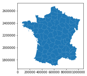
You can simply call function plot() to render the geospatial data as a map on a plot (matplotlib):
>>> gdf.plot()
3.2 Create pygeoda object from geodataframe
pygeoda provides a utility function geopandas_to_geoda to easily create a pygeoda instance for spatial data analysis:
>>> import pygeoda
>>> guerry = pygeoda.open(gdf)
Note
The conversion is based on using Well-Known-Binary (WKB) format to exchange geometric data for good performance.
The function geopandas_to_geoda() returns an object of geoda class, which can be then used to access GeoDa functions to do spatial data analysis. For example, to examine the local Moran of variable “crm_prs” (Population per Crime against persons), we first create a Queen contiguity weights:
>>> queen_w = pygeoda.queen_weights(guerry)
>>> queen_w
Weights Meta-data:
 number of observations:                   85
           is symmetric:                 True
               sparsity:  0.05813148788927336
        # min neighbors:                    2
        # max neighbors:                    8
       # mean neighbors:   4.9411764705882355
     # median neighbors:                  5.0
           has isolates:                Fals
3.3 ESDA with pygeoda and geopandas
Local Moran CLuster Map
Now, with the geoda object guerry, you can call pygeoda’s spatial analysis functions. For example, to examine the local Moran statistics of variable “crm_prs” (Population per Crime against persons):
>>> crm_prp = gdf['Crm_prp']
>>> crm_lisa = pygeoda.local_moran(queen_w, crm_prp)
Now, with the LISA results, we can do exploratory spatial data analysis by generating a LISA cluster map:
import matplotlib
import matplotlib.pyplot as plt

fig, ax = plt.subplots(figsize = (10,10))
lisa_colors = crm_lisa.lisa_colors()
lisa_labels = crm_lisa.lisa_labels()

# attach LISA cluster indicators to geodataframe
gdf['LISA'] = crm_lisa.lisa_clusters()

for ctype, data in gdf.groupby('LISA'):
    color = lisa_colors[ctype]
    lbl = lisa_labels[ctype]
    data.plot(color = color,
        ax = ax,
        label = lbl,
        edgecolor = 'black',
        linewidth = 0.2)

# Place legend in the lower right hand corner of the plot
lisa_legend = [matplotlib.lines.Line2D([0], [0], color=color, lw=2) for color in lisa_colors]
ax.legend(lisa_legend, lisa_labels,loc='lower left', fontsize=12, frameon=True)
ax.set(title='Local Moran Cluster Map of Crm_prp\n Population per Crime against persons')
ax.set_axis_off()
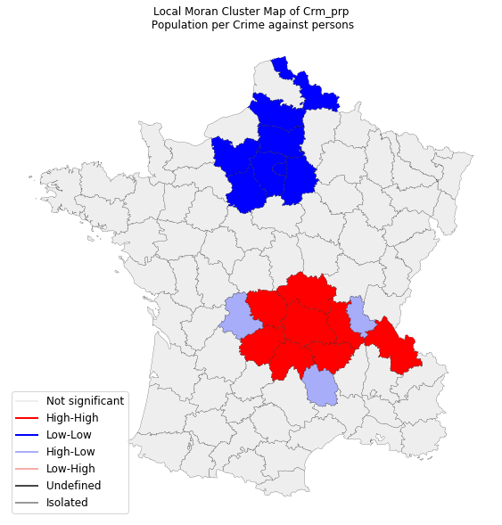
From the above code, you can see that we still use gpf object to do plotting. The values of cluster indicators from pygeoda’s crm_lisa object are used to make the LISA map.This emphasis that pygeoda is a API focused library, which only provides the core functions of spatial data analysis for easy integration.
If you check the values of the cluster indicators, you will see they are integer numbers 0 (not significant), 1 (high-high cluster), 2 (low-low cluster), 3 (low-high cluster), 4 (high-low cluster), 5 (neighborless/island), 6 (undefined), which are excatly the same with GeoDa software when you save LISA results to a table.
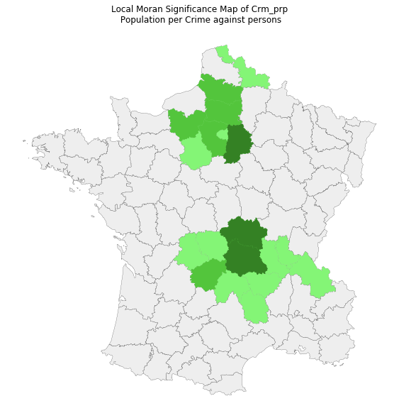
To create a siginificant map that is associated with the Local Moran map:
gdf['LISA_PVAL'] = crm_lisa.lisa_pvalues()
fig, ax = plt.subplots(figsize = (10,10))
gdf.plot(color='#eeeeee', ax=ax, edgecolor = 'black', linewidth = 0.2)
gdf[gdf['LISA_PVAL'] <= 0.05].plot(color="#84f576", ax=ax)
gdf[gdf['LISA_PVAL'] <= 0.01].plot(color="#53c53c", ax=ax)
gdf[gdf['LISA_PVAL'] <= 0.001].plot(color="#348124", ax=ax)
ax.set(title='Local Moran Significance Map of Crm_prp\n Population per Crime against persons')
ax.set_axis_off()
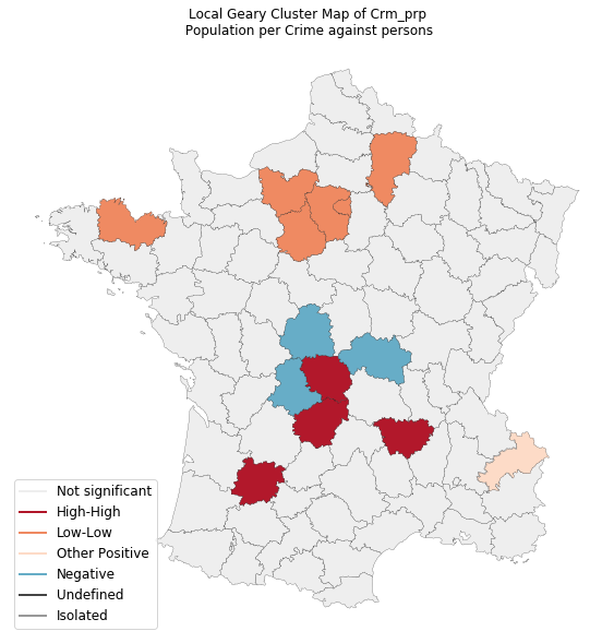
Local Geary Cluster Map
Another example is to create a map of local Geary:
>>> crm_geary = pygeoda.local_geary(queen_w, crm_prp)
Then, use matplotlib to create a local geary map:
fig, ax = plt.subplots(figsize = (10,10))
lisa_colors = crm_geary.lisa_colors()
lisa_labels = crm_geary.lisa_labels()

# attach LISA cluster indicators to geodataframe
gdf['GEARY'] = crm_geary.lisa_clusters()

for ctype, data in gdf.groupby('GEARY'):
    color = lisa_colors[ctype]
    lbl = lisa_labels[ctype]
    data.plot(color = color,
        ax = ax,
        label = lbl,
        edgecolor = 'black',
        linewidth = 0.2)

# Place legend in the lower right hand corner of the plot
lisa_legend = [matplotlib.lines.Line2D([0], [0], color=color, lw=2) for color in lisa_colors]
ax.legend(lisa_legend, lisa_labels,loc='lower left', fontsize=12, frameon=True)
ax.set(title='Local Geary Cluster Map of Crm_prp\n Population per Crime against persons')
ax.set_axis_off()
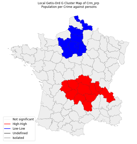
Local G Cluster Map
To create a map of local Getis-Order G:
>>> crm_g = pygeoda.local_g(queen_w, crm_prp)
Then, use matplotlib to create a local geary map:
fig, ax = plt.subplots(figsize = (10,10))
lisa_colors = crm_g.lisa_colors()
lisa_labels = crm_g.lisa_labels()

# attach LISA cluster indicators to geodataframe
gdf['GO'] = crm_g.GetClusterIndicators()

for ctype, data in gdf.groupby('GO'):
    color = lisa_colors[ctype]
    lbl = lisa_labels[ctype]
    data.plot(color = color,
        ax = ax,
        label = lbl,
        edgecolor = 'black',
        linewidth = 0.2)

# Place legend in the lower right hand corner of the plot
lisa_legend = [matplotlib.lines.Line2D([0], [0], color=color, lw=2) for color in lisa_colors]
ax.legend(lisa_legend, lisa_labels,loc='lower left', fontsize=12, frameon=True)
ax.set(title='Local Getis-Ord G Cluster Map of Crm_prp\n Population per Crime against persons')
ax.set_axis_off()