Tutorial of rgeoda

rgeoda is an R library for spatial data analysis. It is an R wrapper of the libgeoda C++ library, which is built based on the GeoDa software. The version used in this tutorial is version 0.0.8.

1. Install `rgeoda`

The rgeoda package can be installed using “install.packages()” command:

install.packages("rgeoda")

, and then can be loaded using the customary “library()” command:

library(rgeoda)

## Loading required package: digest

In addition, the package sf needs to be loaded, since it is a dependency:

library(sf)

## Linking to GEOS 3.11.0, GDAL 3.5.3, PROJ 9.1.0; sf_use_s2() is TRUE

2. Load Spatial Data

The rgeoda package for R relies on the sf (simple features) package for basic spatial data handling functions. In a typical R workflow, one first reads a shape file or other GIS format file with the data using the sf st_read(file path) command. For example, to load the ESRI Shapefile Guerry.shp comes with the package:

guerry_path <- system.file("extdata", "Guerry.shp", package = "rgeoda")
guerry <- st_read(guerry_path)

## Reading layer `Guerry' from data source 
##   `/Users/runner/work/_temp/Library/rgeoda/extdata/Guerry.shp' 
##   using driver `ESRI Shapefile'
## Simple feature collection with 85 features and 29 fields
## Geometry type: MULTIPOLYGON
## Dimension:     XY
## Bounding box:  xmin: 47680 ymin: 1703258 xmax: 1031401 ymax: 2677441
## Projected CRS: NTF (Paris) / Lambert zone II

Once the spatial object has been created, it can be used to compute a spatial weights matrix using one of the several weights functions in rgeoda.

3. Spatial Weights

Spatial weights are central components in spatial data analysis. The spatial weights represent the possible spatial interactions between observations in space. rgeoda provides 6 functions to create 4 different types of spatial weights:

Contiguity Based Weights: queen_weights(), rook_weights()
Distance Based Weights: distance_weights()
K-Nearest Neighbor Weights: knn_weights()
Kernel Weights: distance_weights() and knn_weights() with kernel parameters

3.1 Queen Contiguity Weights

Contiguity means that two spatial units share a common border of non-zero length. Operationally, we can further distinguish between a rook and a queen criterion of contiguity, in analogy to the moves allowed for the such-named pieces on a chess board. The queen criterion is somewhat more encompassing and defines neighbors as spatial units sharing a common edge or a common vertex.

To create a Queen contiguity weights, one can call the function

queen_weights(sf_obj, order=1, include_lower_order = False, precision_threshold = 0)

For example, to create a Queen contiguity weights using the sf object guerry:

queen_w <- queen_weights(guerry)
summary(queen_w)

##                      name              value
## 1 number of observations:                 85
## 2          is symmetric:                TRUE
## 3               sparsity: 0.0581314878892734
## 4        # min neighbors:                  2
## 5        # max neighbors:                  8
## 6       # mean neighbors:   4.94117647058824
## 7     # median neighbors:                  5
## 8           has isolates:              FALSE

The function queen_weights() returns an instance of Weight object. One can access the meta data of the spatial weights by accessing the attributes of GeoDaWeight object:

Attributes of `Weight` object

is_symmetric(queen_w)

## [1] TRUE

has_isolates(queen_w)

## [1] FALSE

weights_sparsity(queen_w)

## [1] 0.05813149

To access the details of the weights: e.g. list the neighbors of a specified observation:

nbrs <- get_neighbors(queen_w, idx = 1)
cat("\nNeighbors of the 1-st observation are:", nbrs)

## 
## Neighbors of the 1-st observation are: 36 37 67 69

To compute the spatial lag of a specified observation by passing the values of the selected variable:

lag <- spatial_lag(queen_w, guerry['Crm_prs'])
lag

##    Spatial.Lag
## 1     23047.50
## 2     26919.67
## 3     26195.50
## 4     14401.25
## 5     15038.67
## 6     15749.00
## 7     22111.67
## 8     13672.33
## 9     22859.20
## 10    11475.20
## 11    12200.14
## 12    13278.67
## 13    24734.00
## 14    11752.83
## 15    17992.60
## 16    21974.40
## 17    26711.00
## 18    19344.00
## 19    23696.71
## 20    25108.67
## 21    21643.17
## 22    18306.00
## 23    24280.00
## 24    14451.60
## 25    21047.67
## 26    21421.33
## 27    25961.50
## 28    10869.83
## 29    13415.67
## 30    17172.17
## 31    20238.25
## 32    12504.25
## 33    26723.00
## 34    21772.83
## 35    26462.20
## 36    19252.00
## 37    24683.20
## 38    20607.25
## 39    24412.00
## 40    19373.71
## 41    16000.20
## 42    23993.25
## 43    20337.86
## 44    16818.67
## 45    17113.83
## 46    13013.00
## 47    22133.00
## 48    24093.75
## 49    25661.67
## 50    22190.17
## 51    29030.00
## 52    16951.00
## 53    24509.00
## 54    24982.75
## 55    19491.50
## 56    24176.00
## 57    27639.67
## 58    21274.33
## 59    24510.33
## 60    30166.00
## 61    23459.00
## 62    16184.00
## 63    18002.00
## 64    10910.00
## 65    16251.25
## 66    15572.00
## 67    25884.25
## 68    23020.60
## 69    26495.00
## 70    24690.50
## 71    17339.00
## 72    25522.33
## 73    18970.00
## 74    19701.83
## 75    21841.00
## 76    24520.40
## 77    14025.80
## 78    14565.17
## 79    13306.67
## 80    12579.00
## 81    21529.50
## 82    23474.50
## 83    24373.17
## 84    19900.50
## 85    23373.60

3.2 Rook Contiguity Weights

The rook criterion defines neighbors by the existence of a common edge between two spatial units. To create a Rook contiguity weights, one can call function:

rook_weights(sf_obj, order=1,include_lower_order=False, precision_threshold = 0)

For example, to create a Rook contiguity weights using the sf object guerry:

rook_w <- rook_weights(guerry)
summary(rook_w)

##                      name              value
## 1 number of observations:                 85
## 2          is symmetric:                TRUE
## 3               sparsity: 0.0581314878892734
## 4        # min neighbors:                  2
## 5        # max neighbors:                  8
## 6       # mean neighbors:   4.94117647058824
## 7     # median neighbors:                  5
## 8           has isolates:              FALSE

The weights we created are in memory. To save the weights to a file, one can call the function:

save_weights(gda_w, id_variable, out_path, layer_name = "")

The id_variable defines the unique value of each observation when saving a weights file

The layer_name is the layer name of loaded dataset. For a ESRI shapefile, the layer name is the file name without the suffix (e.g. Guerry).

For example, using Guerry dataset, the column “CODE_DE” can be used as a key to save a weights file:

save_weights(rook_w, guerry['CODE_DE'], out_path = '/Users/xun/Downloads/Guerry_r.gal', 
             layer_name = 'Guerry')

## [1] FALSE

3.3 Distance Based Weights

The most straightforward spatial weights matrix constructed from a distance measure is obtained when i and j are considered neighbors whenever j falls within a critical distance band from i. In order to start the distance based neighbors, we first need to compute a threshold value. rgeoda provides a function min_distthreshold to help you find a optimized distance threshold that guarantees that every observation has at least one neighbor:

min_distthreshold(GeoDa gda, bool is_arc = False, is_mile = True)
To create a Distance based weights, one can call the function `distance_weights`:

Then, with this distance threshold, we can create a distance-band weights using the function:

distance_weights(geoda_obj, dist_thres, power=1.0,  is_inverse=False, is_arc=False, is_mile=True)

For example:

dist_thres <- min_distthreshold(guerry)
dist_thres

## [1] 96726.14

dist_w <- distance_weights(guerry, dist_thres)
summary(dist_w)

##                      name              value
## 1 number of observations:                 85
## 2          is symmetric:                TRUE
## 3               sparsity: 0.0434602076124567
## 4        # min neighbors:                  1
## 5        # max neighbors:                  7
## 6       # mean neighbors:   3.69411764705882
## 7     # median neighbors:                  4
## 8           has isolates:              FALSE

3.4 K-Nearest Neighbor Weights

A special case of distance based weights is K-Nearest neighbor weights, in which every obersvation will have exactly k neighbors. It can be used to avoid the problem of isolate in distance-band weights when a smaller cut-off distance is used. To create a KNN weights, we can call the function knn_weights:

knn_weights(gda, k, power = 1.0,is_inverse = False, is_arc = False, is_mile = True)

For example, to create a 6-nearest neighbor weights using Guerry:

knn6_w <- knn_weights(guerry, 6)
summary(knn6_w)

##                      name              value
## 1 number of observations:                 85
## 2          is symmetric:               FALSE
## 3               sparsity: 0.0705882352941176
## 4        # min neighbors:                  6
## 5        # max neighbors:                  6
## 6       # mean neighbors:                  6
## 7     # median neighbors:                  6
## 8           has isolates:              FALSE

3.5 Kernel Weights

Kernel weights apply kernel function to determine the distance decay in the derived continuous weights kernel. The kernel weights are defined as a function K(z) of the ratio between the distance dij from i to j, and the bandwidth hi, with z=dij/hi.

The kernel functions include

triangular
uniform
quadratic
epanechnikov
quartic
gaussian

Two functions are provided in rgeoda to create kernel weights.

Use `kernel_weights` for Kernel Weights with adaptive bandwidth

To create a kernel weights with fixed bandwith:

bandwidth <- min_distthreshold(guerry)
kernel_w <- kernel_weights(guerry, bandwidth, kernel_method = "uniform")
summary(kernel_w)

##                      name              value
## 1 number of observations:                 85
## 2          is symmetric:               FALSE
## 3               sparsity: 0.0434602076124567
## 4        # min neighbors:                  1
## 5        # max neighbors:                  7
## 6       # mean neighbors:   3.69411764705882
## 7     # median neighbors:                  4
## 8           has isolates:              FALSE

The arguments is_inverse, power, is_arc and is_mile are the same with the distance based weights. Additionally, kernel_weights has another argument that user can specify:

use_kernel_diagonals    
(optional) FALSE (default) or TRUE, apply kernel on the diagonal of weights matrix

Use `kernel_knn_weights` for Kernel Weights with adaptive bandwidth

To create a kernel weights with adaptive bandwidth or using max Knn distance as bandwidth:

adptkernel_w = kernel_knn_weights(guerry, 6, "uniform")

summary(adptkernel_w)

##                      name              value
## 1 number of observations:                 85
## 2          is symmetric:               FALSE
## 3               sparsity: 0.0705882352941176
## 4        # min neighbors:                  6
## 5        # max neighbors:                  6
## 6       # mean neighbors:                  6
## 7     # median neighbors:                  6
## 8           has isolates:              FALSE

This kernel weights function two more arguments that user can specify:

adaptive_bandwidth  
(optional) TRUE (default) or FALSE: TRUE use adaptive bandwidth calculated using distance of k-nearest neithbors, FALSE use max distance of all observation to their k-nearest neighbors

use_kernel_diagonals    
(optional) FALSE (default) or TRUE, apply kernel on the diagonal of weights matrix

4 Local Indicators of Spatial Association–LISA

rgeoda provides following methods for local spatial autocorrelation statistics:

Local Moran: local_moran(), local_moran_eb()
Local Geary: local_geary(), local_multigeary()
Local Getis-Ord statistics: local_g() and local_gstar()
Local Join Count: local_joincount(), local_bijoincount(), local_multijoincount()
Quantile LISA: local_quantilelisa(), local_multiquantilelisa()
Local Neighbor Match Test: neighbor_match_test()

For more information about the local spatial autocorrelation statisticis, please read Dr. Luc Anselin’s lab notes: http://geodacenter.github.io/workbook/6a_local_auto/lab6a.html.

4.1 Local Moran

The Local Moran statistic is a method to identify local clusters and local spatial outliers. For example, we can call the function local_moran() with the created Queen weights and the data “crm_prp = guerry[‘Crm_prp’]” as input parameters:

crm_prp = guerry["Crm_prp"]
lisa <- local_moran(queen_w, crm_prp)

The local_moran() function will return a lisa object, and we can access its values/results of lisa computation using the following functions:

lisa_clusters(): Get the local cluster indicators returned from LISA computation.
lisa_colors(): Get the cluster colors of LISA computation.
lisa_labels(): Get the cluster labels of LISA computation.
lisa_values(): Get the local spatial autocorrelation values returned from LISA computation.
lisa_num_nbrs(): Get the number of neighbors of every observations in LISA computation.
lisa_pvalues(): Get the local pseudo-p values of significance returned from LISA computation.
lisa_fdr(): Get the False Discovery Rate (FDR) in LISA.
lisa_bo(): Get the False Discovery Rate (FDR) in LISA.

For example, we can call the function lisa_values() to get the values of the local Moran:

lms <- lisa_values(gda_lisa = lisa)
lms

##  [1]  0.0154319783  0.3270633224  0.0212952962  0.0046105448 -0.0028342407
##  [6]  0.4149377158 -0.1379463091  0.0998657692  0.2823176310  0.1218745112
## [11] -0.0951205417  0.0326111938  0.3878324535  1.1888723840 -0.6452792226
## [16] -0.3096492740  0.3662775143  2.0375343539 -0.0050154800  0.0697110572
## [21]  2.2720355722  0.2886391551 -0.0070189726 -0.0009906605  0.9517469793
## [26]  0.7648322095  0.0432039929 -0.0045362842 -0.0964911860  0.0952360887
## [31]  0.0100895206 -0.0109401003 -0.0544245927 -0.0345553975  0.0887531916
## [36]  0.0954232056  0.0383617454 -0.1776714441  0.1638208393  1.2309154898
## [41]  2.9077203402 -0.0396340261  0.4458735227  0.2491123240  0.0905643622
## [46] -0.6212977834 -0.0308773407  0.0375870399  0.2270376112 -0.0918254739
## [51] -0.0112400086  0.1085584763 -0.0055113129 -0.0027097589  0.7235016208
## [56]  0.0163129939  0.4246564560  0.3787307767 -0.0597158189  0.5050011802
## [61]  2.7632125275  0.0656510809  0.1771899330 -0.0572150317  0.4943795537
## [66]  0.2870386197 -1.4593300774 -0.0055305930  0.4895990016 -0.0324125662
## [71]  2.1366499813  0.9041683235  0.7053678641  1.4098290925  0.0051652159
## [76]  0.2238144189 -0.1621373954  0.0195632289 -0.3233724187 -0.0337778226
## [81]  0.0118189869 -0.1164679533 -0.5699624657 -0.0859634996  0.2085373916

To get the pseudo-p values of significance of local Moran computation:

pvals <- lisa_pvalues(lisa)
pvals

##  [1] 0.414 0.123 0.001 0.474 0.452 0.087 0.243 0.326 0.299 0.303 0.237 0.461
## [13] 0.248 0.015 0.178 0.166 0.124 0.003 0.456 0.346 0.053 0.145 0.431 0.425
## [25] 0.005 0.037 0.465 0.395 0.138 0.316 0.495 0.431 0.359 0.129 0.295 0.058
## [37] 0.090 0.231 0.258 0.018 0.026 0.455 0.073 0.057 0.222 0.023 0.369 0.338
## [49] 0.282 0.359 0.483 0.252 0.450 0.434 0.138 0.327 0.063 0.005 0.097 0.292
## [61] 0.001 0.217 0.237 0.126 0.145 0.344 0.008 0.340 0.079 0.300 0.033 0.142
## [73] 0.001 0.001 0.460 0.005 0.212 0.384 0.110 0.409 0.455 0.353 0.006 0.287
## [85] 0.128

To get the cluster indicators of local Moran computation:

cats <- lisa_clusters(lisa, cutoff = 0.05)
cats

##  [1] 0 0 1 0 0 0 0 0 0 0 0 0 0 1 0 0 0 1 0 0 0 0 0 0 2 2 0 0 0 0 0 0 0 0 0 0 0 0
## [39] 0 1 1 0 0 0 0 3 0 0 0 0 0 0 0 0 0 0 0 2 0 0 1 0 0 0 0 0 3 0 0 0 2 0 2 2 0 2
## [77] 0 0 0 0 0 0 3 0 0

The predefined values of the indicators of LISA cluster are:

0 Not significant
1 High-High
2 Low-Low
3 High-Low
4 Low-High
5 Undefined
6 Isolated

which can be accessed via the function lisa_labels():

lbls <- lisa_labels(lisa)
lbls

## [1] "Not significant" "High-High"       "Low-Low"         "Low-High"       
## [5] "High-Low"        "Undefined"       "Isolated"

By default, the local_moran() function will run with some default parameters, e.g.:

significance_cutoff: 0.05
permutation: 999
permutation_method: 'complete'
cpu_threads: 6
seed (for random number generator): 123456789

, which are identical to GeoDa desktop software so to replicate the results in GeoDa software. You can set different values when calling the lisa functions.

For example, re-run the above local Moran example using 9,999 permutations.

lisa <- local_moran(queen_w, crm_prp, permutations = 9999)

Then, we can use the same lisa object to get the new results after 9,999 permutations:

pvals <- lisa_pvalues(lisa)
pvals

##  [1] 0.4186 0.1265 0.0004 0.4679 0.4545 0.0728 0.2313 0.3071 0.3115 0.3087
## [11] 0.2187 0.4834 0.2686 0.0102 0.2024 0.1790 0.1320 0.0020 0.4558 0.3519
## [21] 0.0479 0.1376 0.4441 0.4195 0.0032 0.0388 0.4736 0.4188 0.1277 0.3300
## [31] 0.4939 0.4427 0.3393 0.1419 0.2714 0.0606 0.0724 0.2247 0.2628 0.0185
## [41] 0.0214 0.4899 0.0719 0.0589 0.2288 0.0189 0.3759 0.3216 0.2812 0.3735
## [51] 0.4695 0.2743 0.4518 0.4286 0.1471 0.3221 0.0647 0.0025 0.0917 0.2812
## [61] 0.0001 0.2419 0.2462 0.1266 0.1270 0.3553 0.0094 0.3122 0.0724 0.2975
## [71] 0.0307 0.1320 0.0001 0.0002 0.4633 0.0056 0.2162 0.3681 0.1334 0.4069
## [81] 0.4536 0.3547 0.0035 0.3096 0.1277

rgeoda uses GeoDa C++ code, in which multi-threading is used to accelerate the computation of LISA. We can use the argument ncpu to specify how many threads to run the computation:

lisa <- local_moran(queen_w, crm_prp, cpu_threads = 4)

Get the False Discovery Rate value based on current pseudo-p values:

fdr <- lisa_fdr(lisa, 0.05)
fdr

## [1] 0.0005882353

Then, one can set the FDR value as the cutoff p-value to filter the cluster results:

cat_fdr <- lisa_clusters(lisa, cutoff = fdr)
cat_fdr

##  [1] 0 0 0 0 0 0 0 0 0 0 0 0 0 0 0 0 0 0 0 0 0 0 0 0 0 0 0 0 0 0 0 0 0 0 0 0 0 0
## [39] 0 0 0 0 0 0 0 0 0 0 0 0 0 0 0 0 0 0 0 0 0 0 0 0 0 0 0 0 0 0 0 0 0 0 0 0 0 0
## [77] 0 0 0 0 0 0 0 0 0

4.2 Local Geary

Local Geary is a type of LISA that focuses on squared differences/dissimilarity. A small value of the local geary statistics suggest positive spatial autocorrelation, whereas large values suggest negative spatial autocorrelation. For more details, please read: http://geodacenter.github.io/workbook/6b_local_adv/lab6b.html#local-geary

For example, we can call the function local_geary() with the created Queen weights and the data “crm_prp” as input parameters:

geary_crmprp <- local_geary(queen_w, crm_prp)

To get the cluster indicators of the local Geary computation:

lisa_clusters(geary_crmprp)

##  [1] 0 2 4 0 3 0 0 0 0 0 0 0 0 0 0 0 0 0 0 2 1 0 0 0 2 2 0 0 0 0 0 0 0 4 0 0 0 0
## [39] 0 0 1 0 0 0 1 0 0 0 0 0 3 0 0 0 0 0 0 0 0 0 0 0 0 0 0 0 0 0 0 0 2 0 0 2 0 0
## [77] 0 0 0 0 0 0 4 0 0

To get the pseudo-p values of the local Geary computation:

lisa_pvalues(geary_crmprp)

##  [1] 0.398 0.027 0.025 0.126 0.017 0.314 0.610 0.141 0.284 0.110 0.559 0.456
## [13] 0.211 0.255 0.226 0.211 0.089 0.054 0.182 0.017 0.030 0.216 0.395 0.105
## [25] 0.024 0.033 0.089 0.416 0.504 0.059 0.380 0.254 0.211 0.048 0.113 0.154
## [37] 0.160 0.571 0.310 0.093 0.009 0.130 0.128 0.178 0.039 0.088 0.076 0.319
## [49] 0.291 0.438 0.043 0.464 0.177 0.099 0.100 0.232 0.141 0.317 0.615 0.208
## [61] 0.198 0.299 0.084 0.634 0.148 0.423 0.060 0.108 0.293 0.257 0.032 0.102
## [73] 0.057 0.003 0.706 0.560 0.605 0.066 0.320 0.391 0.175 0.601 0.007 0.365
## [85] 0.238

4.3 Multivariate Local Geary:

To apply multivariate local geary, we need to define a string with the variable names and use this string to extract the relevant subset from the data frame. For example, we apply multivariate local geary on variables “Crm_prs”, “Crm_prp”, “Litercy”, “Donatns”, “Infants” and “Suicids”:

data <-guerry[c('Crm_prs','Crm_prp','Litercy','Donatns','Infants','Suicids')]
multigeary <- local_multigeary(queen_w, data)

To get the cluster indicators of the local Geary computation:

lisa_clusters(multigeary)

##  [1] 0 1 1 1 0 1 1 1 1 1 1 1 0 0 0 0 0 1 1 1 1 1 0 0 1 1 1 1 0 1 0 0 1 0 0 0 0 0
## [39] 1 0 1 2 1 1 1 0 0 0 1 1 1 0 1 1 0 0 1 1 0 1 1 0 1 0 1 1 0 1 0 1 1 0 1 1 0 1
## [77] 1 1 1 1 0 1 0 1 1

4.4 Local Getis-Ord Statistics

There are two types of local Getis-Ord statistics: one is computing a ratio of the weighted average of the values in the neighboring locations, not including the value at the location; while another type of statistic includes the value at the location in both numerator and denominator. For more details, please read: http://geodacenter.github.io/workbook/6b_local_adv/lab6b.html#getis-ord-statistics

A value larger than the mean suggests a high-high cluster or hot spot, a value smaller than the mean indicates a low-low cluster or cold spot.

For example, we can call the function local_g() with the created Queen weights and the data “crm_prp” as input parameters:

localg_crmprp <- local_g(queen_w, crm_prp)

To get the cluster indicators of the local G computation:

lisa_clusters(localg_crmprp)

##  [1] 0 0 1 0 0 0 0 0 0 0 0 0 0 1 0 0 0 1 0 0 0 0 0 0 2 2 0 0 0 0 0 0 0 0 0 0 0 0
## [39] 0 1 1 0 0 0 0 1 0 0 0 0 0 0 0 0 0 0 0 2 0 0 1 0 0 0 0 0 1 0 0 0 2 0 2 2 0 2
## [77] 0 0 0 0 0 0 1 0 0

To get the pseudo-p values of the local G computation:

lisa_pvalues(localg_crmprp)

##  [1] 0.414 0.123 0.001 0.474 0.452 0.087 0.243 0.326 0.299 0.303 0.237 0.461
## [13] 0.248 0.015 0.178 0.166 0.124 0.003 0.456 0.346 0.053 0.145 0.432 0.425
## [25] 0.005 0.037 0.464 0.395 0.138 0.316 0.495 0.431 0.359 0.129 0.295 0.058
## [37] 0.090 0.231 0.258 0.018 0.026 0.455 0.073 0.057 0.222 0.023 0.369 0.338
## [49] 0.282 0.359 0.483 0.252 0.450 0.434 0.138 0.327 0.063 0.005 0.097 0.292
## [61] 0.001 0.217 0.237 0.127 0.145 0.344 0.008 0.340 0.079 0.300 0.033 0.142
## [73] 0.001 0.001 0.461 0.005 0.212 0.384 0.110 0.409 0.455 0.353 0.006 0.287
## [85] 0.128

For the second type of local Getis-Ord statistics, we can call the function local_gstar() with the created Queen weights and the data “crm_prp” as input parameters:

localgstar_crmprs <- local_gstar(queen_w, crm_prp)
lisa_pvalues(localgstar_crmprs)

##  [1] 0.414 0.123 0.001 0.474 0.452 0.087 0.243 0.326 0.299 0.303 0.237 0.461
## [13] 0.248 0.015 0.178 0.166 0.124 0.003 0.456 0.346 0.053 0.145 0.432 0.425
## [25] 0.005 0.037 0.464 0.395 0.138 0.316 0.495 0.431 0.359 0.129 0.295 0.058
## [37] 0.090 0.231 0.258 0.018 0.026 0.455 0.073 0.057 0.222 0.023 0.369 0.338
## [49] 0.282 0.359 0.483 0.252 0.450 0.434 0.138 0.327 0.063 0.005 0.097 0.292
## [61] 0.001 0.217 0.237 0.127 0.145 0.344 0.008 0.340 0.079 0.300 0.033 0.142
## [73] 0.001 0.001 0.461 0.005 0.212 0.384 0.110 0.409 0.455 0.353 0.006 0.287
## [85] 0.128

4.5 Local Join Count

Local Join Count is a method to identify local clusters for binary data by using a local version of the so-called BB join count statistic. The statistic is only meaningful for those observations with value 1. For more details, please read http://geodacenter.github.io/workbook/6d_local_discrete/lab6d.html

For example, we can call the function local_joincount() with a Queen weights and the data “TopCrm”, which is a set of binary (0,1) values, as input parameters:

top_crm <- guerry['TopCrm']
localjc_crm <- local_joincount(queen_w, top_crm)

To get the pseudo-p values of the local Join Count computation:

lisa_pvalues(localjc_crm)

##  [1] 0.395 0.085 0.094    NA    NA    NA 0.255    NA    NA    NA    NA    NA
## [13]    NA    NA    NA    NA    NA    NA 0.170 0.242 0.394    NA    NA    NA
## [25]    NA    NA 0.111    NA    NA    NA    NA    NA    NA 0.095    NA    NA
## [37] 0.189    NA    NA 0.284    NA    NA    NA    NA    NA    NA 0.218 0.378
## [49]    NA 0.367 0.037 0.233 0.174 0.392    NA 0.282 0.028 0.370 0.298 0.106
## [61]    NA    NA    NA    NA    NA    NA    NA    NA 0.009 0.325    NA    NA
## [73]    NA    NA    NA 0.041    NA    NA    NA    NA    NA    NA    NA    NA
## [85]    NA

To get the cluster indicators of the local Join Count computation:

lisa_clusters(localjc_crm)

##  [1] 0 0 0 0 0 0 0 0 0 0 0 0 0 0 0 0 0 0 0 0 0 0 0 0 0 0 0 0 0 0 0 0 0 0 0 0 0 0
## [39] 0 0 0 0 0 0 0 0 0 0 0 0 1 0 0 0 0 0 1 0 0 0 0 0 0 0 0 0 0 0 1 0 0 0 0 0 0 1
## [77] 0 0 0 0 0 0 0 0 0

To get the number of neighbors of the local Join Count computation:

lisa_num_nbrs(localjc_crm)

##  [1] 4 6 6 4 3 7 3 3 5 5 7 3 3 6 5 5 6 6 7 3 6 7 2 5 6 6 2 6 6 6 4 4 6 6 5 6 5 4
## [39] 6 7 5 4 7 6 6 5 8 4 6 6 5 4 5 4 2 6 3 6 6 2 6 3 3 2 4 2 4 5 7 6 2 3 8 6 5 5
## [77] 5 6 3 6 4 6 6 6 5

4.6 Bivariate and Multivariate Local Join Count:

Bivariate Local Join Count means, in a bivariate local join count, the two events cannot happen in the same location. It is also called “no-colocation” join count. To demonstrate this function, we manually create a new variable:

inv_crm <- 1 - as.data.frame(guerry[,"TopCrm"])[,1] # create no-location case
guerry['Inv_Crm'] <- inv_crm

Now, top_crm and inv_crm are no-colocation bivariate cases. Then, we apply the local_bijoicount():

jc <- local_bijoincount(queen_w, guerry[c('TopCrm', 'Inv_Crm')])

In case of co-location, a warning message will be raised “The bivariate local join count only applies on two variables with no-colocation.” , and one can use pygeoda.local_multijoincount() for co-location case.

To get the cluster indicators of the multivariate local join count computation:

lisa_pvalues(jc)

##  [1] 0.106 0.013 0.017    NA    NA    NA 0.035    NA    NA    NA    NA    NA
## [13]    NA    NA 0.135    NA    NA    NA 0.040 0.024 0.296    NA    NA    NA
## [25]    NA    NA    NA    NA    NA    NA 0.208    NA    NA 0.398    NA    NA
## [37] 0.047    NA    NA 0.407    NA    NA    NA    NA    NA    NA 0.487 0.098
## [49]    NA 0.292 0.007 0.416 0.035 0.101    NA 0.076    NA 0.305 0.086    NA
## [61]    NA    NA    NA    NA    NA    NA    NA    NA 0.001 0.100    NA    NA
## [73]    NA    NA    NA 0.005    NA    NA    NA    NA    NA    NA    NA    NA
## [85]    NA

To get the cluster indicators of the local Join Count computation:

lisa_clusters(jc)

##  [1] 0 1 1 0 0 0 1 0 0 0 0 0 0 0 0 0 0 0 1 1 0 0 0 0 0 0 0 0 0 0 0 0 0 0 0 0 1 0
## [39] 0 0 0 0 0 0 0 0 0 0 0 0 1 0 1 0 0 0 0 0 0 0 0 0 0 0 0 0 0 0 1 0 0 0 0 0 0 1
## [77] 0 0 0 0 0 0 0 0 0

Co-location Local Join Count is for where two or more events happen in the same location. Therefore, the function local_multijoincount takes a list of variables with 0/1 values as the input parameter:

bin_data <- guerry[c('TopWealth','TopWealth', 'TopLit')] 
jc <- local_multijoincount(queen_w, bin_data)

To get the cluster indicators of the multivariate local join count computation:

lisa_pvalues(jc)

##  [1]    NA    NA    NA 0.256 0.205    NA    NA    NA    NA    NA    NA    NA
## [13]    NA    NA    NA    NA    NA    NA    NA    NA    NA    NA    NA    NA
## [25]    NA    NA    NA    NA    NA    NA    NA    NA    NA    NA    NA    NA
## [37] 0.319    NA    NA    NA    NA    NA    NA    NA    NA    NA    NA    NA
## [49]    NA    NA    NA    NA    NA    NA    NA    NA    NA    NA    NA    NA
## [61]    NA 0.175 0.192    NA    NA    NA    NA 0.051    NA    NA    NA    NA
## [73]    NA    NA    NA    NA    NA    NA    NA    NA    NA    NA    NA 0.348
## [85]    NA

4.7 Quantile LISA

The quantile local spatial autocorrelation converte the continuous variable to a binary variable that takes the value of 1 for a specific quantile. Then appaly a local join count to the data converted. Two input parameters, k and q, need to be specified in the function pygeoda.quantile_lisa(): k is the number of quantiles (k > 2), and the q is the index of selected quantile lisa ranging from 1 to k.

For example, the examples in section 4.1.5 can be simply implemented as

qsa <- local_quantilelisa(queen_w, crm_prp, 5, 5)

To get the p-values and cluster indicators of the quantile LISA computation:

lisa_pvalues(qsa)

##  [1] 0.419    NA    NA    NA    NA 0.376    NA 0.442    NA 0.257    NA    NA
## [13]    NA 0.082 0.348    NA 0.277 0.010    NA    NA 0.090 0.387    NA    NA
## [25]    NA    NA    NA    NA    NA 0.271    NA 0.447    NA    NA    NA    NA
## [37]    NA    NA    NA 0.026 0.003    NA    NA    NA    NA    NA    NA    NA
## [49]    NA    NA    NA    NA    NA    NA    NA    NA    NA    NA    NA    NA
## [61] 0.001    NA 0.465    NA    NA    NA    NA    NA 0.378    NA    NA    NA
## [73]    NA    NA    NA    NA    NA    NA    NA    NA    NA    NA    NA    NA
## [85]    NA

lisa_clusters(qsa)

##  [1] 0 0 0 0 0 0 0 0 0 0 0 0 0 0 0 0 0 1 0 0 0 0 0 0 0 0 0 0 0 0 0 0 0 0 0 0 0 0
## [39] 0 1 1 0 0 0 0 0 0 0 0 0 0 0 0 0 0 0 0 0 0 0 1 0 0 0 0 0 0 0 0 0 0 0 0 0 0 0
## [77] 0 0 0 0 0 0 0 0 0

Multivariate Quantile LISA

For multiple variables, the Quantile LISA can automatiaclly detect if it is the case of no-colocation, in which local_bijoincount() will be called internally, or the case of co-location, in which local_multijoincount() will be called internally.

qsa <- local_multiquantilelisa(queen_w, guerry[c("TopCrm", "TopLit")], c(5,5), c(5,5))

To get the p-values and cluster indicators of the quantile LISA computation:

lisa_pvalues(qsa)

##  [1]    NA 0.122    NA    NA    NA    NA 0.023    NA    NA    NA    NA    NA
## [13]    NA    NA    NA    NA    NA    NA 0.137    NA    NA    NA    NA    NA
## [25]    NA    NA    NA    NA    NA    NA    NA    NA    NA    NA    NA    NA
## [37] 0.412    NA    NA    NA    NA    NA    NA    NA    NA    NA    NA    NA
## [49]    NA 0.111    NA 0.323 0.012    NA    NA    NA    NA 0.465    NA    NA
## [61]    NA    NA    NA    NA    NA    NA    NA    NA    NA    NA    NA    NA
## [73]    NA    NA    NA    NA    NA    NA    NA    NA    NA    NA    NA    NA
## [85]    NA

lisa_clusters(qsa)

##  [1] 0 0 0 0 0 0 1 0 0 0 0 0 0 0 0 0 0 0 0 0 0 0 0 0 0 0 0 0 0 0 0 0 0 0 0 0 0 0
## [39] 0 0 0 0 0 0 0 0 0 0 0 0 0 0 1 0 0 0 0 0 0 0 0 0 0 0 0 0 0 0 0 0 0 0 0 0 0 0
## [77] 0 0 0 0 0 0 0 0 0

4.8 Bivariate Local Moran

The bivariate Local Moran’s I captures the relationship between the value for one variable at location i, and the average of the neighboring values for another variable. Please note this statistic needs to be interpreted with caution, since it ignores in-situ correlation between the two variables. The most meaningful application of the bivariate Local Moran statistic is comparing the same variable at two time periods. See: https://geodacenter.github.io/workbook/6c_local_multi/lab6c.html#bivariate-local-moran

qsa <- local_bimoran(queen_w, guerry[c('Crm_prs', 'Litercy')])

5 Spatial Clustering

Spatial clustering aims to group of a large number of geographic areas or points into a smaller number of regions based on similiarities in one or more variables. Spatially constrained clustering is needed when clusters are required to be spatially contiguous.

There are three different approaches explicitly incorporate the contiguity constraint in the optimization process: SKATER, Redcap and Max-p. For more details, please read: * http://geodacenter.github.io/workbook/9c_spatial3/lab9c.html * http://geodacenter.github.io/workbook/9d_spatial4/lab9d.html

For example, to apply spatial clustering on the Guerry dataset, we use the queen weights to define the spatial contiguity and select 6 variables for similarity measure: “Crm_prs”, “Crm_prp”, “Litercy”, “Donatns”, “Infants”, “Suicids”.

data <- guerry[c('Crm_prs','Crm_prp','Litercy','Donatns','Infants','Suicids')]

5.1 SKATER

The Spatial C(K)luster Analysis by Tree Edge Removal(SKATER) algorithm introduced by Assuncao et al. (2006) is based on the optimal pruning of a minimum spanning tree that reflects the contiguity structure among the observations. It provides an optimized algorithm to prune to tree into several clusters that their values of selected variables are as similar as possible.

The rgeoda’s SKATER function is:

skater(k, w, data, distance_method='euclidean', bound_vals = [],  min_bound = 0, random_seed=123456789)

For example, to create 4 spatially contiguous clusters using Guerry dataset, the queen weights and the values of the 6 selected variables:

guerry_clusters <- skater(4, queen_w, data)
guerry_clusters

## $Clusters
##  [1] 3 2 3 1 1 1 2 1 2 1 1 1 2 1 1 3 3 3 2 4 3 1 2 1 2 2 4 1 1 1 1 1 4 3 4 1 2 1
## [39] 4 3 3 4 2 1 1 1 4 4 2 2 4 2 2 4 2 3 2 2 4 2 3 1 1 1 2 2 1 2 3 4 2 2 2 2 3 2
## [77] 1 1 1 1 3 3 3 2 2
## 
## $`Total sum of squares`
## [1] 504
## 
## $`Within-cluster sum of squares`
## [1] 57.89077 59.95242 28.72571 69.38030 62.30781 66.65809
## 
## $`Total within-cluster sum of squares`
## [1] 159.0849
## 
## $`The ratio of between to total sum of squares`
## [1] 0.3156447

This skater() function returns a names list with names “Clusters”, “Total sum of squares”, “Within-cluster sum of squares”, “Total within-cluster sum of squares”, and “The ratio of between to total sum of squares”.

5.2 REDCAP

REDCAP (Regionalization with dynamically constrained agglomerative clustering and partitioning) is developed by D. Guo (2008). Like SKATER, REDCAP starts from building a spanning tree in 3 different ways (single-linkage, average-linkage, and the complete-linkage). The single-linkage way leads to build a minimum spanning tree. Then, REDCAP provides 2 different ways (first-order and full-order constraining) to prune the tree to find clusters. The first-order approach with a minimum spanning tree is the same as SKATER. In GeoDa and rgeoda, the following methods are provided:

First-order and Single-linkage
Full-order and Complete-linkage
Full-order and Average-linkage
Full-order and Single-linkage
Full-order and Wards-linkage

For example, to find 4 clusters using the same dataset and weights as above using REDCAP with Full-order and Complete-linkage method:

redcap_clusters <- redcap(4, queen_w, data, "fullorder-completelinkage")
redcap_clusters

## $Clusters
##  [1] 1 2 1 3 3 1 2 3 2 3 3 3 2 1 1 1 1 1 2 1 1 1 2 3 2 2 1 3 3 3 3 3 1 1 1 3 2 3
## [39] 1 1 4 1 2 3 3 3 1 1 2 2 1 2 2 1 2 1 2 2 1 2 1 3 3 3 2 2 3 2 1 1 2 2 2 2 1 2
## [77] 3 3 3 3 1 1 1 2 2
## 
## $`Total sum of squares`
## [1] 504
## 
## $`Within-cluster sum of squares`
## [1] 59.33033 55.01580 28.20272 68.58974 61.27232 54.63519
## 
## $`Total within-cluster sum of squares`
## [1] 176.9539
## 
## $`The ratio of between to total sum of squares`
## [1] 0.351099

5.3 Spatially Constrained Hierarchical Clucstering

Spatially constrained hierarchical clustering is a special form of constrained clustering, where the constraint is based on contiguity (common borders). The method builds up the clusters using agglomerative hierarchical clustering methods: single linkage, complete linkage, average linkage and Ward’s method (a special form of centroid linkage). Meanwhile, it also maintains the spatial contiguity when merging two clusters.

For example, to find 4 spatially constrained clusters using the same dataset and weights as above using Complete-linkage method:

schc_clusters <- schc(4, queen_w, data, "complete")
schc_clusters

## $Clusters
##  [1] 1 1 1 1 1 1 1 1 1 1 1 1 4 1 1 1 1 1 1 1 3 1 1 1 1 1 1 1 1 1 1 1 1 1 1 1 1 1
## [39] 1 1 2 1 1 1 1 1 1 1 1 1 1 1 1 1 1 1 1 1 1 1 1 1 1 1 1 1 1 1 1 1 1 1 1 1 1 1
## [77] 1 1 1 1 1 1 1 1 1
## 
## $`Total sum of squares`
## [1] 504
## 
## $`Within-cluster sum of squares`
## [1] 78.13831 54.75868 81.49771 63.48675 80.60111 65.74389
## 
## $`Total within-cluster sum of squares`
## [1] 79.77355
## 
## $`The ratio of between to total sum of squares`
## [1] 0.1582809

5.4 AZP

The automatic zoning procedure (AZP) was initially outlined in Openshaw (1977) as a way to address some of the consequences of the modifiable areal unit problem (MAUP). In essence, it consists of a heuristic to find the best set of combinations of contiguous spatial units into p regions, minimizing the within-sum of squares as a criterion of homogeneity. The number of regions needs to be specified beforehand, as in most other clustering methods considered so far.

rgeoda provides three different heuristic algorithms to find an optimal solution for AZP:

greedy
Tabu Search
Simulated Annealing

5.4.1 AZP greedy

The original AZP heuristic is a local optimization procedure that cycles through a series of possible swaps between spatial units at the boundary of a set of regions. The process starts with an initial feasible solution, i.e., a grouping of n spatial units into p contiguous regions. This initial solution can be constructed in several different ways. The initial solution must satisfy the contiguity constraints. For example, this can be accomplished by growing a set of contiguous regions from p randomly selected seed units by adding neighboring locations until the contiguity constraint can no longer be met.

azp_clusters <- azp_greedy(5, queen_w, data)
azp_clusters

## $Clusters
##  [1] 5 2 3 1 1 1 2 1 2 1 1 1 2 1 4 4 3 4 2 3 3 1 2 1 2 2 3 1 1 1 1 1 3 3 3 1 2 1
## [39] 2 3 1 3 2 1 1 1 3 3 2 2 3 2 2 3 2 3 2 2 3 2 1 1 1 1 2 2 1 2 3 3 2 2 2 2 4 2
## [77] 1 1 1 1 4 4 4 2 2
## 
## $`Total sum of squares`
## [1] 504
## 
## $`Within-cluster sum of squares`
## [1] 47.20703 60.10165 32.71213 57.69760 59.41673 65.49840
## 
## $`Total within-cluster sum of squares`
## [1] 181.3665
## 
## $`The ratio of between to total sum of squares`
## [1] 0.3598541

5.4.2 AZP Simulated Annealing

To call AZP simulate annealing algorithm, one needs to specify cooling_rate (default: 0.85):

azp_clusters <- azp_sa(5, queen_w, data, cooling_rate = 0.85)
azp_clusters

## $Clusters
##  [1] 5 2 3 1 1 1 2 1 2 1 1 1 2 1 4 4 3 4 2 3 3 1 2 1 2 2 3 1 1 1 1 1 3 3 3 1 2 1
## [39] 3 3 1 3 2 1 1 1 3 3 2 2 3 2 2 3 2 3 2 2 3 2 1 1 1 1 2 2 1 2 3 3 2 2 2 2 4 2
## [77] 1 1 1 1 4 4 4 2 2
## 
## $`Total sum of squares`
## [1] 504
## 
## $`Within-cluster sum of squares`
## [1] 47.86263 61.08506 29.62824 58.04068 60.31298 66.23291
## 
## $`Total within-cluster sum of squares`
## [1] 180.8375
## 
## $`The ratio of between to total sum of squares`
## [1] 0.3588045

5.4.3 AZP Tabu Search

To call AZP Tabu search algorithm, one needs to specify tabu_length (deafult: 10) , or conv_tabu (default: 10):

azp_clusters <- azp_tabu(5, queen_w, data, tabu_length = 10, conv_tabu = 10)
azp_clusters

## $Clusters
##  [1] 4 1 2 3 3 3 1 3 1 3 3 3 2 4 2 2 2 2 1 2 4 2 1 3 1 1 2 3 3 3 2 3 2 2 2 3 1 2
## [39] 2 4 4 2 1 3 2 3 2 2 1 1 2 1 1 2 1 2 1 1 2 1 4 3 3 3 1 1 3 1 4 2 1 1 1 1 5 1
## [77] 3 3 3 3 5 5 2 1 1
## 
## $`Total sum of squares`
## [1] 504
## 
## $`Within-cluster sum of squares`
## [1] 52.20796 39.86439 30.75532 54.95106 54.00440 59.41931
## 
## $`Total within-cluster sum of squares`
## [1] 212.7976
## 
## $`The ratio of between to total sum of squares`
## [1] 0.4222174

NOTE: the AZP algorithm is very sensitive to the initial positions for constructing final solutions. Therefore, the random seed, which is used to determine the initial positions, could be used to execute several rounds of max-p algorithms for sensitive analysis.

5.5 Max-p

The so-called max-p regions model (outlined in Duque, Anselin, and Rey 2012) uses a different approach and considers the regionalization problem as an application of integer programming. Besides, the number of regions is determined endogenously.

The algorithm itself consists of a search process that starts with an initial feasible solution and iteratively improves upon it while maintaining contiguity among the elements of each cluster. rgeoda provides three different heuristic algorithms to find an optimal solution for max-p:

greedy
Tabu Search
Simulated Annealing

Unlike SKATER and REDCAP that one can specify the number of clusters as an input parameter, max-p doesn’t allow to specify the number of clusters explicitly, but a constrained variable and the minimum bounding value that each cluster should reach that are used to find an optimized number of clusters.

5.5.1 Max-p greedy

For example, to use the greedy algorithm in maxp function with the same dataset and weights as above to find optimal clusters using max-p:

First, we need to specify, for example, every cluster must have population >= 3236.67 thousand people:

bound_vals <- guerry['Pop1831']
min_bound <- 3236.67 # 10% of Pop1831

Then, we can call the max-p function with the “greedy” algorithm, the bound values, and minimum bound value:

maxp_clusters <- maxp_greedy(queen_w, data, bound_vals, min_bound)
maxp_clusters

## $Clusters
##  [1] 7 2 7 1 1 1 2 3 6 3 1 1 8 7 4 4 5 7 2 4 7 3 6 1 8 8 4 1 3 3 3 1 4 5 5 7 2 3
## [39] 5 7 7 4 8 1 3 1 5 5 6 6 5 6 2 4 6 5 2 2 5 8 7 3 3 3 6 6 2 6 2 5 8 8 2 8 4 8
## [77] 1 1 1 1 4 4 4 6 2
## 
## $`Total sum of squares`
## [1] 504
## 
## $`Within-cluster sum of squares`
## [1] 44.39253 37.80089 28.19168 53.09362 48.11754 48.21628
## 
## $`Total within-cluster sum of squares`
## [1] 244.1875
## 
## $`The ratio of between to total sum of squares`
## [1] 0.4844989

Note: the results of max-p may be different with GeoDa desktop software, it is caused by the different implementation of boost::unordered_map in version 1.58 (used in GeoDa) and version 1.75 (used in rgeoda via BH package). The keys in boost::unordered_map are not ordered and have different orders in the two Boost versions we used. This involves a different mechanism of randomness in max-p algorithm when picking which area or region to process. Therefore, the results might be slightly different. This is normal and shows the sensitiveness of the max-p algorithm: see https://geodacenter.github.io/workbook/9d_spatial4/lab9d.html#max-p-region-problem for more about sensitivy study of max-p algorithm.

If you want to replicate the identical results as in GeoDa software v1.18.0, please install BH == 1.58.0-1 and build/install rgeoda from source using: devtools::install_github("lixun910/rgeoda")

5.5.2 Max-p Tabu Search

To use tabu search algorithm in maxp function, we can specify the parameters of tabu_length and conv_tabu:

maxp_tabu_clusters <- maxp_tabu(queen_w, data, bound_vals, min_bound, tabu_length=10, conv_tabu=10)
maxp_tabu_clusters

## $Clusters
##  [1] 2 5 1 3 3 1 5 1 4 1 1 3 6 1 2 7 2 7 5 8 2 7 4 3 6 6 8 3 1 1 7 3 8 2 7 3 5 7
## [39] 2 2 1 8 6 1 7 3 2 2 4 5 8 4 4 8 4 2 5 5 2 6 1 1 1 1 4 4 3 4 2 2 6 6 5 6 2 6
## [77] 1 1 3 3 8 7 7 4 5
## 
## $`Total sum of squares`
## [1] 504
## 
## $`Within-cluster sum of squares`
## [1] 37.71292 53.00122 24.16448 61.51004 53.23544 33.45476
## 
## $`Total within-cluster sum of squares`
## [1] 240.9211
## 
## $`The ratio of between to total sum of squares`
## [1] 0.4780181

5.5.3 Max-p Simulated Annealing

To apply simulated annealing algorithm in maxp function with the parameter of cooling rate:

maxp_sa_clusters <- maxp_sa(queen_w, data, bound_vals, min_bound, cooling_rate=0.85, sa_maxit=1)
maxp_sa_clusters

## $Clusters
##  [1] 2 3 7 5 5 7 3 1 6 1 7 5 8 7 4 4 2 7 3 4 7 7 6 5 8 8 4 5 1 1 1 5 4 2 2 5 3 1
## [39] 2 7 7 4 8 1 1 5 2 2 6 6 2 6 3 4 6 2 3 3 2 3 7 1 1 1 6 6 5 6 2 2 8 8 3 8 4 3
## [77] 1 1 5 5 4 4 4 6 3
## 
## $`Total sum of squares`
## [1] 504
## 
## $`Within-cluster sum of squares`
## [1] 44.78939 44.22570 24.40716 52.89492 50.78755 36.79676
## 
## $`Total within-cluster sum of squares`
## [1] 250.0985
## 
## $`The ratio of between to total sum of squares`
## [1] 0.4962272

We can also increase the number of iterations for local search process by specifying the parameter iterations (default value is 99):

maxp_clusters <- maxp_greedy(queen_w, data, bound_vals, min_bound, iterations=199)
maxp_clusters

## $Clusters
##  [1] 7 2 7 1 1 1 2 3 6 3 1 1 8 7 4 4 5 7 2 4 7 3 6 1 8 8 4 1 3 3 3 1 4 5 5 7 2 3
## [39] 5 7 7 4 8 1 3 1 5 5 6 6 5 6 2 4 6 5 2 2 5 8 7 3 3 3 6 6 2 6 2 5 8 8 2 8 4 8
## [77] 1 1 1 1 4 4 4 6 2
## 
## $`Total sum of squares`
## [1] 504
## 
## $`Within-cluster sum of squares`
## [1] 44.39253 37.80089 28.19168 53.09362 48.11754 48.21628
## 
## $`Total within-cluster sum of squares`
## [1] 244.1875
## 
## $`The ratio of between to total sum of squares`
## [1] 0.4844989

NOTE: the max-p algorithm is very sensitive to the initial positions for constructing final solutions. Therefore, the random seed, which is used to determine the initial positions, could be used to execute several rounds of max-p algorithms for sensitive analysis.

6 Exploratory Spatial Data Analysis

For exploratory spatial data analysis (ESDA), rgeoa provides some utility functions to allow users to easily work with sf to visualize the results and do exploratory spatial data analysis.

6.1 Start from `sf` package

The sf package has been popular tool to handle geospatial data. It is a good substitue of sp package which will be deprecated soon.

For example, we can simply call plot() function to render the first 9 chorepleth maps using the frist 9 variables in the dataset:

plot(guerry)

## Warning: plotting the first 9 out of 30 attributes; use max.plot = 30 to plot
## all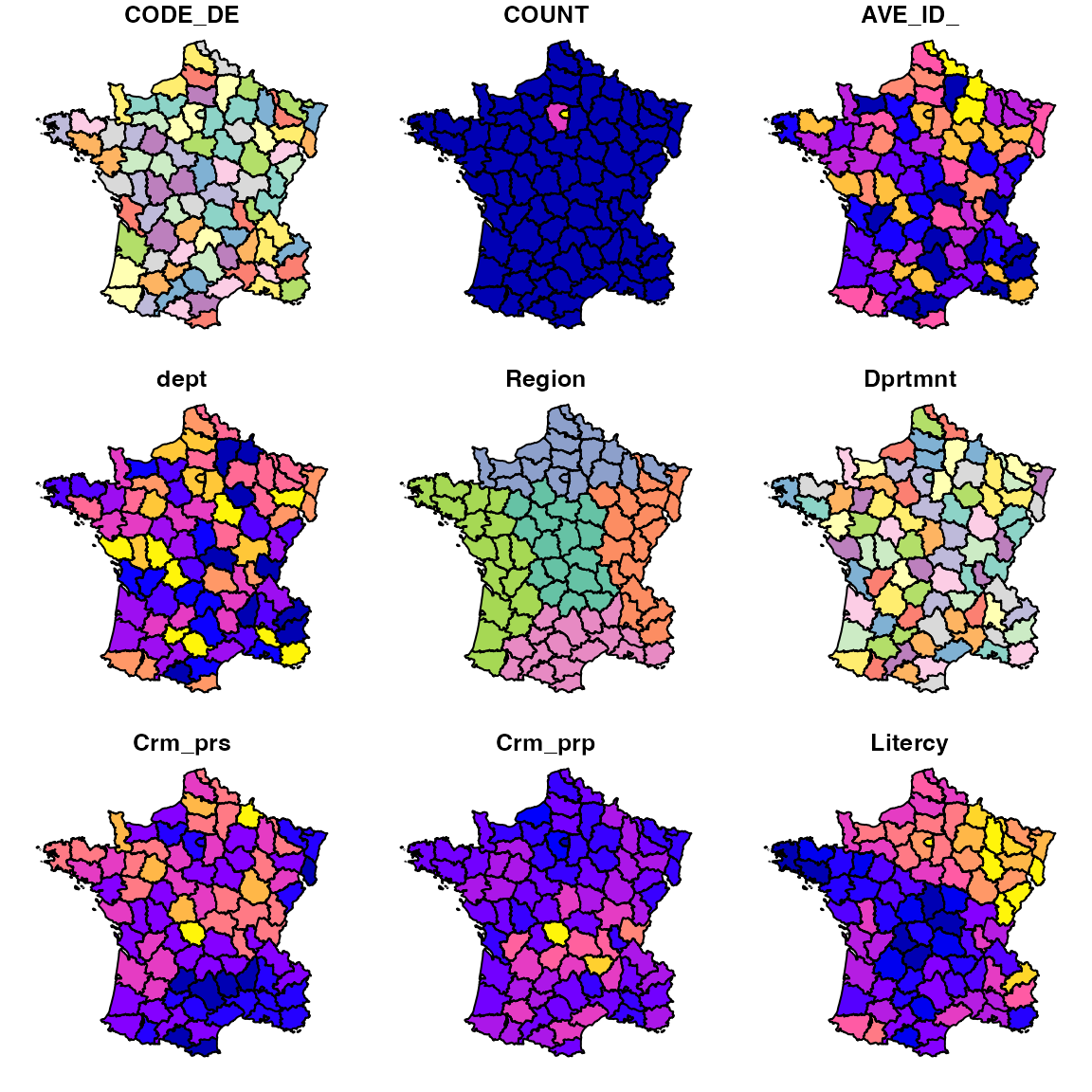

6.2 ESDA with rgeoda

Now, with the sf object guerry, you can call rgeoda’s spatial analysis functions. For example, to examine the local Moran statistics of variable “crm_prs” (Population per Crime against persons):

queen_w <- queen_weights(guerry)
lisa <- local_moran(queen_w,  guerry['Crm_prs'])

Note: rgeoda uses wkb, which is a binary representation of geometries, to exchange data between sf and libgeoda in memory.

6.3 Create Local Moran Map

With the LISA results, we can make a local moran cluster map:

lisa_colors <- lisa_colors(lisa)
lisa_labels <- lisa_labels(lisa)
lisa_clusters <- lisa_clusters(lisa)

plot(st_geometry(guerry), 
     col=sapply(lisa_clusters, function(x){return(lisa_colors[[x+1]])}), 
     border = "#333333", lwd=0.2)
title(main = "Local Moran Map of Crm_prs")
legend('bottomleft', legend = lisa_labels, fill = lisa_colors, border = "#eeeeee")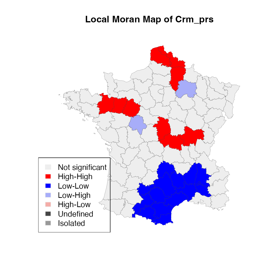

In the above code, we use th values of cluster indicators from rgeoda’s LISA object are used to make the LISA map. We can save the clusters back to the original sf data.frame:

guerry['moran_cluster'] <- lisa_clusters

Checking the values of the cluster indicators, we will see they are integer numbers 0 (not significant), 1 (high-high cluster), 2 (low-low cluster), 3 (low-high cluster), 4 (high-low cluster), 5 (neighborless/island), 6 (undefined):

lisa_clusters

##  [1] 0 1 1 0 0 2 0 2 0 2 2 0 0 2 0 0 1 0 0 0 0 0 0 2 0 0 0 2 2 0 0 2 1 0 3 0 0 0
## [39] 0 0 0 0 0 0 0 2 0 0 3 0 1 0 0 0 0 0 1 0 0 1 0 0 0 2 0 0 0 0 1 1 0 0 0 0 0 0
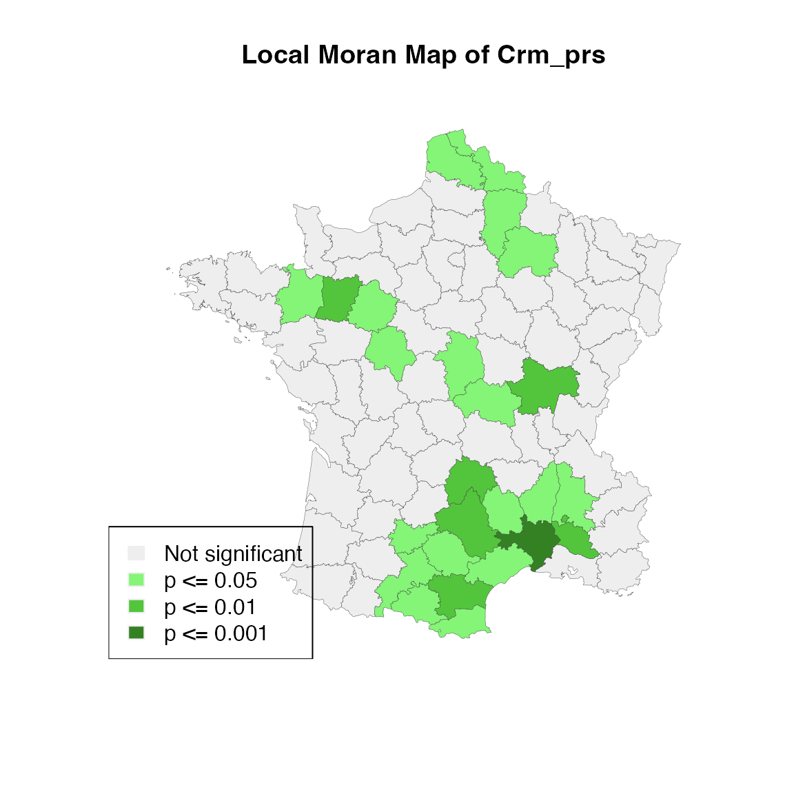
## [77] 2 2 0 2 0 0 0 0 0

To create a significance map that is associated with the local Moran map, we can do the same as making the local moran cluster map using the results from lisa_pvalues():

lisa_p <- lisa_pvalues(lisa)
p_labels <- c("Not significant", "p <= 0.05", "p <= 0.01", "p <= 0.001")
p_colors <- c("#eeeeee", "#84f576", "#53c53c", "#348124")
plot(st_geometry(guerry), 
     col=sapply(lisa_p, function(x){
       if (x <= 0.001) return(p_colors[4])
       else if (x <= 0.01) return(p_colors[3])
       else if (x <= 0.05) return (p_colors[2])
       else return(p_colors[1])
       }), 
     border = "#333333", lwd=0.2)
title(main = "Local Moran Map of Crm_prs")
legend('bottomleft', legend = p_labels, fill = p_colors, border = "#eeeeee")

Xun Li

1/6/2021

1. Install `rgeoda`

2. Load Spatial Data

3. Spatial Weights

3.1 Queen Contiguity Weights

Attributes of `Weight` object

3.2 Rook Contiguity Weights

3.3 Distance Based Weights

3.4 K-Nearest Neighbor Weights

3.5 Kernel Weights

Use `kernel_weights` for Kernel Weights with adaptive bandwidth

Use `kernel_knn_weights` for Kernel Weights with adaptive bandwidth

4 Local Indicators of Spatial Association–LISA

4.1 Local Moran

4.2 Local Geary

4.3 Multivariate Local Geary:

4.4 Local Getis-Ord Statistics

4.5 Local Join Count

4.6 Bivariate and Multivariate Local Join Count:

4.7 Quantile LISA

4.8 Bivariate Local Moran

5 Spatial Clustering

5.1 SKATER

5.2 REDCAP

5.3 Spatially Constrained Hierarchical Clucstering

5.4 AZP

5.4.1 AZP greedy

5.4.2 AZP Simulated Annealing

5.4.3 AZP Tabu Search

5.5 Max-p

5.5.1 Max-p greedy

5.5.2 Max-p Tabu Search

5.5.3 Max-p Simulated Annealing

6 Exploratory Spatial Data Analysis

6.1 Start from `sf` package

6.2 ESDA with rgeoda

6.3 Create Local Moran Map

Tutorial of rgeoda

Xun Li

1/6/2021

1. Install rgeoda

2. Load Spatial Data

3. Spatial Weights

3.1 Queen Contiguity Weights

Attributes of Weight object

3.2 Rook Contiguity Weights

3.3 Distance Based Weights

3.4 K-Nearest Neighbor Weights

3.5 Kernel Weights

Use kernel_weights for Kernel Weights with adaptive bandwidth

Use kernel_knn_weights for Kernel Weights with adaptive bandwidth

4 Local Indicators of Spatial Association–LISA

4.1 Local Moran

4.2 Local Geary

4.3 Multivariate Local Geary:

4.4 Local Getis-Ord Statistics

4.5 Local Join Count

4.6 Bivariate and Multivariate Local Join Count:

4.7 Quantile LISA

4.8 Bivariate Local Moran

5 Spatial Clustering

5.1 SKATER

5.2 REDCAP

5.3 Spatially Constrained Hierarchical Clucstering

5.4 AZP

5.4.1 AZP greedy

5.4.2 AZP Simulated Annealing

5.4.3 AZP Tabu Search

5.5 Max-p

5.5.1 Max-p greedy

5.5.2 Max-p Tabu Search

5.5.3 Max-p Simulated Annealing

6 Exploratory Spatial Data Analysis

6.1 Start from sf package

6.2 ESDA with rgeoda

6.3 Create Local Moran Map

1. Install `rgeoda`

Attributes of `Weight` object

Use `kernel_weights` for Kernel Weights with adaptive bandwidth

Use `kernel_knn_weights` for Kernel Weights with adaptive bandwidth

6.1 Start from `sf` package